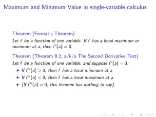
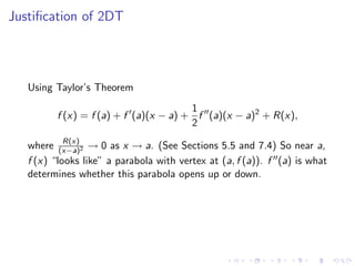
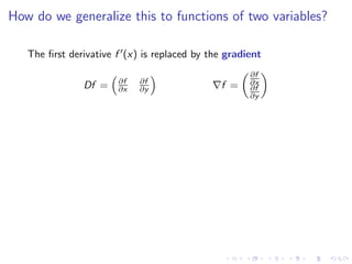
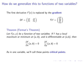
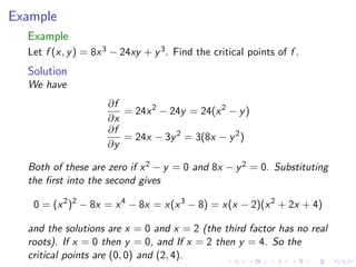
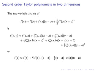
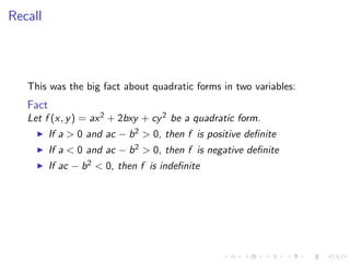
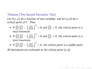
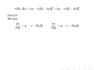
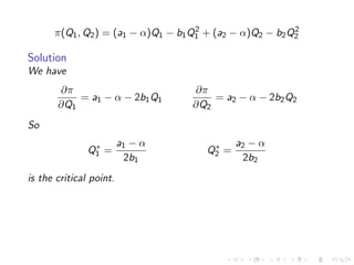
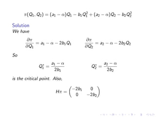
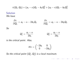
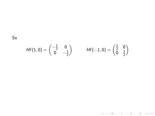
This document summarizes key concepts in unconstrained optimization of functions with two variables, including: 1) Critical points are found by taking the partial derivatives and setting them equal to zero, generalizing the first derivative test for single-variable functions. 2) The Hessian matrix generalizes the second derivative, with its entries being the partial derivatives evaluated at a critical point. 3) The second derivative test classifies critical points as local maxima, minima or saddle points based on the signs of the Hessian matrix's eigenvalues. 4) Taylor polynomial approximations in two variables involve partial derivatives up to second order, analogous to single-variable Taylor series. 5) An example classifies the critical points

1. Lesson 25 (Chapter 17)
Unconstrained Optimization I
Math 20
November 19, 2007
Announcements
Problem Set 9 on the website. Due November 21.
There will be class November 21 and homework due
November 28.
next OH: Monday 1-2pm, Tuesday 3-4pm
Midterm II: Thursday, 12/6, 7-8:30pm in Hall A.

2. Outline
Single-variable recollections
From one to two dimensions
Critical points
The Hessian
The second derivative test
More examples
The discriminating monopolist

3. Maximum and Minimum Value in single-variable calculus
Theorem (Fermat’s Theorem)
Let f be a function of one variable. If f has a local maximum or
minimum at a, then f (a) = 0.

4. Maximum and Minimum Value in single-variable calculus
Theorem (Fermat’s Theorem)
Let f be a function of one variable. If f has a local maximum or
minimum at a, then f (a) = 0.
Theorem (Theorem 9.2, a/k/a The Second Derivative Test)
Let f be a function of one variable, and suppose f (a) = 0.
If f (a) > 0, then f has a local minimum at a.
If f (a) < 0, then f has a local maximum at a.
(If f (a) = 0, this theorem has nothing to say).

5. Justification of 2DT
Using Taylor’s Theorem
1
f (x) = f (a) + f (a)(x − a) + f (a)(x − a)2 + R(x),
2
R(x)
where (x−a)2 → 0 as x → a. (See Sections 5.5 and 7.4) So near a,
f (x) “looks like” a parabola with vertex at (a, f (a)). f (a) is what
determines whether this parabola opens up or down.

6. Outline
Single-variable recollections
From one to two dimensions
Critical points
The Hessian
The second derivative test
More examples
The discriminating monopolist

7. How do we generalize this to functions of two variables?
The first derivative f (x) is replaced by the gradient
∂f
∂f ∂f ∂x
Df = f= ∂f
∂x ∂y
∂y

8. How do we generalize this to functions of two variables?
The first derivative f (x) is replaced by the gradient
∂f
∂f ∂f ∂x
Df = f= ∂f
∂x ∂y
∂y
Theorem (Fermat’s Theorem)
Let f (x, y ) be a function of two variables. If f has a local
maximum or minimum at (a, b), and is differentiable at (a,b), then
∂f ∂f
(a, b) = 0 (a, b) = 0
∂x ∂y
As in one variable, we’ll call these points critical points.

9. Example
Example
Let f (x, y ) = 8x 3 − 24xy + y 3 . Find the critical points of f .

10. Example
Example
Let f (x, y ) = 8x 3 − 24xy + y 3 . Find the critical points of f .
Solution
We have
∂f
= 24x 2 − 24y = 24(x 2 − y )
∂x
∂f
= 24x − 3y 2 = 3(8x − y 2 )
∂y
Both of these are zero if x 2 − y = 0 and 8x − y 2 = 0. Substituting
the first into the second gives
0 = (x 2 )2 − 8x = x 4 − 8x = x(x 3 − 8) = x(x − 2)(x 2 + 2x + 4)
and the solutions are x = 0 and x = 2 (the third factor has no real
roots). If x = 0 then y = 0, and If x = 2 then y = 4. So the
critical points are (0, 0) and (2, 4).

11. How do we generalize this to functions of two variables?
The second derivative f (x) is replaced by . . .

12. How do we generalize this to functions of two variables?
The second derivative f (x) is replaced by . . . a matrix, the
Hessian of f : 2
∂2f

∂f
2
Hf =  ∂x ∂x∂y 


 ∂2f ∂2f 
∂y 2
∂y ∂x

13. Compare and contrast the Hessians at (0, 0) for these functions:
(i) f (x, y ) = x 2 + y 2
(ii) f (x, y ) = 1 − x 2 − y 2
(iii) f (x, y ) = x 2 − y 2
(iv) f (x, y ) = xy
How are they alike and how are they different?

14. Compare and contrast the Hessians at (0, 0) for these functions:
(i) f (x, y ) = x 2 + y 2
(ii) f (x, y ) = 1 − x 2 − y 2
(iii) f (x, y ) = x 2 − y 2
(iv) f (x, y ) = xy
How are they alike and how are they different?
20 20
(i) Hf = (iii) Hf =
0 −2
02
−2 0 01
(ii) Hf = (iv) Hf =
0 −2 10

15. Outline
Single-variable recollections
From one to two dimensions
Critical points
The Hessian
The second derivative test
More examples
The discriminating monopolist

16. Second order Taylor polynomials in two dimensions
The two-variable analog of
1
f (x) ≈ f (a) + f (a)(x − a) + f (a)(x − a)2
2
is
f (x, y ) ≈ f (a, b) + fx (a, b)(x − a) + fy (a, b)(y − b)
+ 2 fxx (a, b)(x − a)2 + fxy (a, b)(x − a)(y − b)
1
+ 1 fyy (a, b)(y − a)2
2
or
1
f (x) ≈ f (a) + f (a) · (x − a) + 2 (x − a) · H(a)(x − a)

17. Recall
This was the big fact about quadratic forms in two variables:
Fact
Let f (x, y ) = ax 2 + 2bxy + cy 2 be a quadratic form.
If a > 0 and ac − b 2 > 0, then f is positive definite
If a < 0 and ac − b 2 > 0, then f is negative definite
If ac − b 2 < 0, then f is indefinite

18. Theorem (The Second Derivative Test)
Let f (x, y ) be a function of two variables, and let (a, b) be a
critical point of f . Then
2
2 2 2 ∂2f
If ∂xf2 ∂yf2 − ∂x∂y
∂∂ ∂f
> 0 and > 0, the critical point is a
∂x 2
local minimum.
2
2 2 2 ∂2f
If ∂xf2 ∂yf2 − ∂x∂y
∂∂ ∂f
> 0 and < 0, the critical point is a
∂x 2
local maximum.
2
∂2f ∂2f ∂2f
−
If < 0, the critical point is a saddle point.
∂x 2 ∂y 2 ∂x∂y
All derivatives are evaluated at the critical point (a, b).

19. Return to the example
Let f (x, y ) = 8x 3 − 24xy + y 3 . Classify the critical points.
∂2f ∂2f
= −24
= 48x
∂x 2 ∂x∂y
∂2f ∂2f
= −24 = 6y
∂y 2
∂y ∂x

20. Return to the example
Let f (x, y ) = 8x 3 − 24xy + y 3 . Classify the critical points.
∂2f ∂2f
= −24
= 48x
∂x 2 ∂x∂y
∂2f ∂2f
= −24 = 6y
∂y 2
∂y ∂x
−24
0
Hf (0, 0) = , which has negative determinant.
−24 0
Hence (0, 0) is a saddle point.
4 −1
Hf (2, 4) = 24 which, since the determinant is
−1 1
positive and the top left entry is positive, indicates a local
minimum.

21. Plotting the function
10
5
0
5
5
10
2
0 0
2
4

22. Plotting the function
5
4
3
2
10
5
1
0
5
5
10
0
2
0 0
2
-1
-1 1
0 2 3
4

23. Online Demo
Try this site (thanks to Tony Pino):
http://www.slu.edu/classes/maymk/banchoff/LevelCurve.html
Launch the applet and enter:
f (x, y ) = x^3 - 3 * x * y + y^3/8 (1/3 of f from the
example)
x from −1 to 10 in 50 steps
y from −1 to 10 in 50 steps
z from −10 to 10 in 50 steps

24. Remarks
The Hessian matrix will always be symmetric in our cases.
If the Hessian has determinant zero, nothing can be said from
this theorem:
f (x, y ) = x 4 + y 4 has a local min at (0, 0)
f (x, y ) = −x 4 − y 4 has a local max at (0, 0)
f (x, y ) = x 4 − y 4 has a saddle point at (0, 0)
±12x 2 0
In each case Hf (x, y ) = , so Hf (0, 0) is the
±12y 2
0
zero matrix.

25. Outline
Single-variable recollections
From one to two dimensions
Critical points
The Hessian
The second derivative test
More examples
The discriminating monopolist

26. Example
A firm sells a product in two separate areas with distinct linear
demand curves, and has monopoly power to decide how much to
sell in each area. How does its maximal profit depend on the
demand in each area?

27. Example
A firm sells a product in two separate areas with distinct linear
demand curves, and has monopoly power to decide how much to
sell in each area. How does its maximal profit depend on the
demand in each area?
Let the demand curves be given by
P1 = a1 − b1 Q1 P2 = a2 − b2 Q2
And the cost function by C = α(Q1 + Q2 ). The profit is therefore
π = P1 Q1 + P2 Q2 − α(Q1 + Q2 )
= (a1 − b1 Q1 )Q1 + (a2 − b2 Q2 )Q2 − α(Q1 + Q2 )
2 2
= (a1 − α)Q1 − b1 Q1 + (a2 − α)Q2 − b2 Q2

28. 2 2
π(Q1 , Q2 ) = (a1 − α)Q1 − b1 Q1 + (a2 − α)Q2 − b2 Q2
Solution

29. 2 2
π(Q1 , Q2 ) = (a1 − α)Q1 − b1 Q1 + (a2 − α)Q2 − b2 Q2
Solution
We have
∂π ∂π
= a1 − α − 2b1 Q1 = a2 − α − 2b2 Q2
∂Q1 ∂Q2

30. 2 2
π(Q1 , Q2 ) = (a1 − α)Q1 − b1 Q1 + (a2 − α)Q2 − b2 Q2
Solution
We have
∂π ∂π
= a1 − α − 2b1 Q1 = a2 − α − 2b2 Q2
∂Q1 ∂Q2
So
a1 − α a2 − α
∗ ∗
Q1 = Q2 =
2b1 2b2
is the critical point.

31. 2 2
π(Q1 , Q2 ) = (a1 − α)Q1 − b1 Q1 + (a2 − α)Q2 − b2 Q2
Solution
We have
∂π ∂π
= a1 − α − 2b1 Q1 = a2 − α − 2b2 Q2
∂Q1 ∂Q2
So
a1 − α a2 − α
∗ ∗
Q1 = Q2 =
2b1 2b2
is the critical point. Also,
−2b1 0
Hπ =
−2b2
0

32. 2 2
π(Q1 , Q2 ) = (a1 − α)Q1 − b1 Q1 + (a2 − α)Q2 − b2 Q2
Solution
We have
∂π ∂π
= a1 − α − 2b1 Q1 = a2 − α − 2b2 Q2
∂Q1 ∂Q2
So
a1 − α a2 − α
∗ ∗
Q1 = Q2 =
2b1 2b2
is the critical point. Also,
−2b1 0
Hπ =
−2b2
0
∗ ∗
So the critical point (Q1 , Q2 ) is a local maximum.

33. Example
x
Find the critical points of f (x, y ) = and classify them.
x 2 +y 2 +1

34. Example
x
Find the critical points of f (x, y ) = and classify them.
x 2 +y 2 +1
Solution
The derivatives are
1 − x2 + y2 2xy
fy = −
fx =
(1 + x 2 + y 2 )2 (1 + x 2 + y 2 )2

35. Example
x
Find the critical points of f (x, y ) = and classify them.
x 2 +y 2 +1
Solution
The derivatives are
1 − x2 + y2 2xy
fy = −
fx =
(1 + x 2 + y 2 )2 (1 + x 2 + y 2 )2
The only way these can both be zero is if y = 0 and x = ±1.

36. Example
x
Find the critical points of f (x, y ) = and classify them.
x 2 +y 2 +1
Solution
The derivatives are
1 − x2 + y2 2xy
fy = −
fx =
(1 + x 2 + y 2 )2 (1 + x 2 + y 2 )2
The only way these can both be zero is if y = 0 and x = ±1. The
second derivatives are
2x x 2 − 3 y 2 + 1 2y −3x 2 + y 2 + 1
fxx = fxy =
(x 2 + y 2 + 1)3 (x 2 + y 2 + 1)3
2 x 3 − 3y 2 x + x
fyy = −
(x 2 + y 2 + 1)3

37. So
−1 1
0 0
2 2
Hf (1, 0) = Hf (−1, 0) =
−1 1
0 0
2 2

38. So
−1 1
0 0
2 2
Hf (1, 0) = Hf (−1, 0) =
−1 1
0 0
2 2
So we have a local max and a local min.

39. Plotting the function
0.5
2
0.0
1
0.5
0
2
1
1
0
1
2
2

40. Plotting the function
2
1
0
0.5
2
0.0
1
-1
0.5
0
2
1
1
0
1
-2
2 -1 1
-2 0 2
2