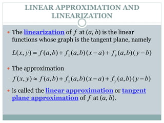
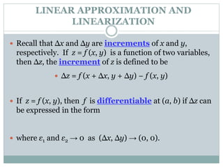
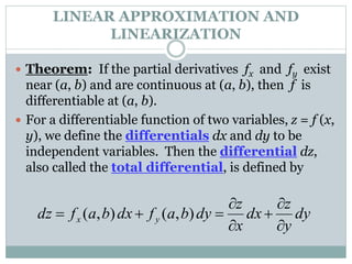
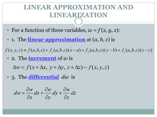
The document discusses concepts related to partial differentiation and its applications. It covers topics like tangent planes, linear approximations, differentials, Taylor expansions, maxima and minima problems, and the Lagrange method. Specifically, it defines the tangent plane to a surface at a point using partial derivatives, describes how to find the linear approximation of functions, and explains how to find maximum and minimum values of functions using critical points and the second derivative test.

1. APPLICATION OF PARTIAL
DIFFERENTIATION

2. Tangent Planes and
Linear Approximations
 Suppose a surface S has equation z = f (x, y), where f has
continuous first partial derivatives, and let P(x0, y0, z0) be a
point on S. Let C1 and C2 be the two curves obtained by
intersection the vertical planes y = y0 and x = x0 with the
surface. Thus, point P lies on both C1 and C2. Let T1 and T2
be the tangent lines to the curves C1 and C2 at point P. Then
the tangent plane to the surface S at point P is defined to
be the plane that contains both tangent lines T1 and T2.

3. Tangent Planes and
Linear Approximations
 Suppose a surface S has equation z = f(x, y), where f
has continuous first partial derivatives.
 Let P(x0, y0, z0) be a point on S.
 We know from Equation that any plane passing
through the point
P(x0, y0, z0) has an equation of the form
)(),()(),( 0000000 yyyxfxxyxfzz yx 

4. LINEAR APPROXIMATION AND
LINEARIZATION
 The linearization of f at (a, b) is the linear
functions whose graph is the tangent plane, namely
 The approximation
 is called the linear approximation or tangent
plane approximation of f at (a, b).
)(),()(),(),(),( bybafaxbafbafyxL yx 
)(),()(),(),(),( bybafaxbafbafyxf yx 

5. LINEAR APPROXIMATION AND
LINEARIZATION
 Recall that Δx and Δy are increments of x and y,
respectively. If z = f (x, y) is a function of two variables,
then Δz, the increment of z is defined to be
 Δz = f (x + Δx, y + Δy) − f (x, y)
 If z = f (x, y), then f is differentiable at (a, b) if Δz can
be expressed in the form
 where ε1 and ε2 → 0 as (Δx, Δy) → (0, 0).

6. LINEAR APPROXIMATION AND
LINEARIZATION
 Theorem: If the partial derivatives fx and fy exist
near (a, b) and are continuous at (a, b), then f is
differentiable at (a, b).
 For a differentiable function of two variables, z = f (x,
y), we define the differentials dx and dy to be
independent variables. Then the differential dz,
also called the total differential, is defined by
dy
y
z
dx
x
z
dybafdxbafdz yx





 ),(),(

7. LINEAR APPROXIMATION AND
LINEARIZATION
 For a function of three variables, w = f (x, y, z):
 1. The linear approximation at (a, b, c) is
 2. The increment of w is
 3. The differential dw is
)(),,()(),,()(),,(),,(),,( czcbafbycbafaxcbafcbafzyxf zyx 
),,(),,( zyxfzzyyxxfw 
dz
z
w
dy
y
w
dx
x
w
dw










8. TAYLOR’s EXPANSIONS
 Let a function be given as the sum of a power
series in the convergence interval of the power series
 Then such a power series is unique and its
coefficients are given by the formula

 f x
   0
0
n
n
n
f x a x x


 
 
 0
!
n
n
f x
a
n


9. TAYLOR’s EXPANSIONS
 If a function has derivatives of all orders at x0,
then we can formally write the corresponding Taylor
series
 The power series created in this way is then called
the Taylor series of the function . A Taylor
series for is called MacLaurin series.
 f x
   
 
 
 
 
 
 
2 30 0 0
0 0 0 0
' '' '''
1! 2! 3!
f x f x f x
f x f x x x x x x x       
 f x
0 0x 

10. TAYLOR’s EXPANSIONS
 There are functions f (x)
 whose formally generated Taylor series do not converge to it.
 A condition that guarantees that this will not happen says that
 the derivatives of f (x) are all uniformly bounded
 in a neighbourhood of x0.

11. TAYLOR’s EXPANSIONS
 There are functions with a Taylor series that, as a
power series, converges to quite a different function
as the following example shows:
Example
   2
1
for 0, 0 0x
f x e x f

  

12. TAYLOR’s EXPANSIONS
0x 
 
2
2
2
1
1
13
3
2 2
'
x
x
x
d e
f x e
dx x
x e


 
 
   
and for x = 0:
 
2
2 2
2 2
1
1 10 0 0
1
0 1 1
' lim lim lim lim lim 0
2
x
t tx x x t t
x x
e txf x
x e te
xe e

    

     

13. TAYLOR’s EXPANSIONS
In a similar way, we could also show that
       
 0 0 ' 0 '' 0 0
k
f f f f     
This means that the Taylor series corresponding to f (x) converges to a
constant function that is equal to zero at all points. But clearly, for
any .
2
1
0x
e

 0x 

14. TAYLOR’s EXPANSIONS
Taylor series of some functions:
2 3
1
1! 2! 3!
x x x x
e     
3 5 7
sin
3! 5! 7!
x x x
x x    
2 4 6
cos 1
2! 4! 6!
x x x
x     
 
2 3 4
ln 1
2 3 4
x x x
x x     

15. Maxima and Minima
 The Least and the Greatest
 Many problems that arise in mathematics call for
finding the largest and smallest values that a
differentiable function can assume on a particular
domain.
 There is a strategy for solving these applied
problems.

16. Maxima and Minima
 The Max-Min Theorem for Continuous Functions
 If f is a continuous function at every point of a
closed interval [a.b], then f takes on a minimum
value, m, and a maximum value, M, on [a,b].
 In other words, a function that is continuous on a
closed interval takes on a maximum and a minimum
on that interval.

17. Maxima and Minima
 The Max-Min Theorem, Graphically

18. Maxima and Minima
 Strategy for Max-Min Problems
 The main problem is setting up the equation:
 Draw a picture. Label the parts that are important for
the problem. Keep track of what the variables represent.
 Use a known formula for the quantity to be maximized or
minimized.
 Write an equation. Try to express the quantity that is to
be maximized or minimized as a function of a single
variable, say y=f (x). This may require some algebra and
the use of information from the problem.

19. Maxima and Minima
 Find an interval of values for this variable. You need
to be mindful of the domain based on restrictions in
the problem.
 Test the critical points and the endpoints. The
extreme value of f will be found among the values f
takes at the endpoints of the domain and at the points
where the derivative is zero or fails to exist.
 List the values of f at these points. If f has an
absolute maximum or minimum on its domain, it will
appear on the list. You may have to examine the sign
pattern of the derivative or the sign of the second
derivative to decide whether a given value represents a
max, min or neither.

20. LAGRANGE METHOD
 Many times a stationary value of the function of
several variables which are not all independent but
connected by some relationship is needed to be
known. Generally, we do convert the given functions
to the one, having least number of independent
variables with the help of these relations, then it
solved. But this not always be necessary to solve such
functions using this ordinary method, and when this
procedure become impractical, Lagrange’s method
proves to be very convenient, which is explained in
the ongoing lines.

21. LAGRANGE METHOD
 Let be a function of three variables which are
connected by the relation
 For u to be have stationary value, it is necessary that
 Also the differential of the relationship function

22. LAGRANGE METHOD
 Multiply (2) by parameter λ and add to (1). Then we
obtain the expression
 To satisfy this equation the components of the expression
need to be equal to zero, i.e.
 This three equations together with the relationship
function i.e. will determine the value of and λ for
which u is stationary.

23. REFERENCE
 http://www.haverford.edu/physics/MathAppendices
/Taylor_Series.pdf
 https://www.google.co.in/webhp?sourceid=chrome-
instant&rlz=1C1GIGM_enIN583IN586&ion=1&espv
=2&ie=UTF-8#q=TAYLOR+EXPANSIONS+PPT
 CALCULUS
 Dr.K.R.Kachot
 Mahajan publishing house