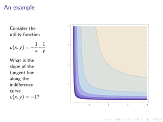
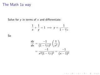
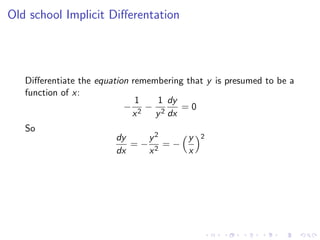
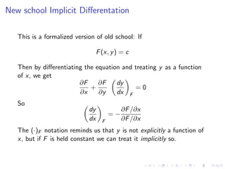
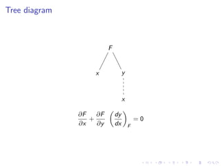
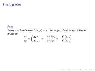
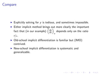
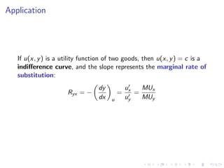
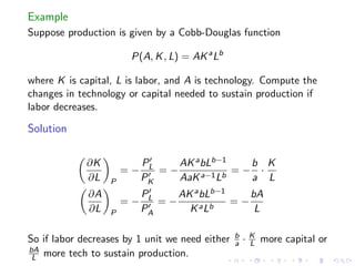
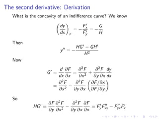
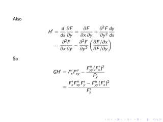
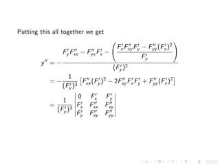
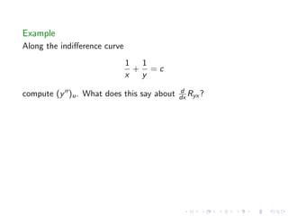
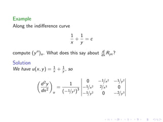
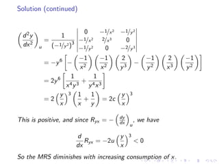
RE Capital's Visionary Leadership under Newman Leech
Lesson24 Implicit Differentiation Slides
1. Lesson 24 (Sections 16.3, 16.7)
Implicit Differentiation
Math 20
November 16, 2007
Announcements
Problem Set 9 on the website. Due November 21.
There will be class November 21 and homework due
November 28.
next OH: Monday 1-2pm, Tuesday 3-4pm
Midterm II: Thursday, 12/6, 7-8:30pm in Hall A.
Go Harvard! Beat Yale!
2. Outline
Cleanup on Leibniz Rule
Implicit Differentiation in two dimensions
The Math 1a way
Old school Implicit Differentation
New school Implicit Differentation
Compare
Application
More than two dimensions
The second derivative
3. Last Time: the Chain Rule
Theorem (The Chain Rule, General Version)
Suppose that u is a differentiable function of the n variables
x1 , x2 , . . . , xn , and each xi is a differentiable function of the m
variables t1 , t2 , . . . , tm . Then u is a function of t1 , t2 , . . . , tm and
∂u ∂u ∂x1 ∂u ∂x2 ∂u ∂xn
= + + ··· +
∂ti ∂x1 ∂ti ∂x2 ∂ti ∂xn ∂ti
4. Last Time: the Chain Rule
Theorem (The Chain Rule, General Version)
Suppose that u is a differentiable function of the n variables
x1 , x2 , . . . , xn , and each xi is a differentiable function of the m
variables t1 , t2 , . . . , tm . Then u is a function of t1 , t2 , . . . , tm and
∂u ∂u ∂x1 ∂u ∂x2 ∂u ∂xn
= + + ··· +
∂ti ∂x1 ∂ti ∂x2 ∂ti ∂xn ∂ti
In summation notation
n
∂u ∂u ∂xj
=
∂ti ∂xj ∂ti
j=1
5. Leibniz’s Formula for Integrals
Fact
Suppose that f (, t, x), a(t), and b(t) are differentiable functions,
and let
b(t)
F (t) = f (t, x) dx
a(t)
6. Leibniz’s Formula for Integrals
Fact
Suppose that f (, t, x), a(t), and b(t) are differentiable functions,
and let
b(t)
F (t) = f (t, x) dx
a(t)
Then
b(t)
∂f (t, x)
F (t) = f (t, b(t))b (t) − f (t, a(t))a (t) + dx
a(t) ∂t
7. Leibniz’s Formula for Integrals
Fact
Suppose that f (, t, x), a(t), and b(t) are differentiable functions,
and let
b(t)
F (t) = f (t, x) dx
a(t)
Then
b(t)
∂f (t, x)
F (t) = f (t, b(t))b (t) − f (t, a(t))a (t) + dx
a(t) ∂t
Proof.
Apply the chain rule to the function
v
H(t, u, v ) = f (t, x) dx
u
with u = a(t) and v = b(t).
10. More about the proof
v
H(t, u, v ) = f (t, x) dx
u
Then by the Fundamental Theorem of Calculus (see Section 10.1)
∂H ∂H
= f (t, v ) = −f (t, u)
∂v ∂u
11. More about the proof
v
H(t, u, v ) = f (t, x) dx
u
Then by the Fundamental Theorem of Calculus (see Section 10.1)
∂H ∂H
= f (t, v ) = −f (t, u)
∂v ∂u
Also,
v
∂H ∂f
= (t, x) dx
∂t u ∂x
since t and x are independent variables.
12. Since F (t) = H(t, a(t), b(t)),
dF ∂H ∂H du ∂H dv
= + +
dt ∂t ∂u dt ∂v dt
b(t)
∂f
= (t, x) + f (t, b(t))b (t) − f (t, a(t))a (t)
a(t) ∂x
13. Application
Example (Example 16.8 with better notation)
Let the profit of a firm be π(t). The present value of the future
profit π(τ ) where τ > t is
π(τ )e −r (τ −t) ,
where r is the discount rate. On a time interval [0, T ], the present
value of all future profit is
T
V (t) = π(τ )e −r (τ −t) dt.
t
Find V (t).
14. Application
Example (Example 16.8 with better notation)
Let the profit of a firm be π(t). The present value of the future
profit π(τ ) where τ > t is
π(τ )e −r (τ −t) ,
where r is the discount rate. On a time interval [0, T ], the present
value of all future profit is
T
V (t) = π(τ )e −r (τ −t) dt.
t
Find V (t).
Answer.
V (t) = rV (t) − π(t)
15. Solution
Since the upper limit is a constant, the only boundary term comes
from the lower limit:
T
∂
V (t) = −π(t)e −r (t−t) + π(τ )e −r τ e rt dτ
t ∂t
T
= −π(t) + r π(τ )e −r τ e rt dτ
t
= rV (t) − π(t).
This means that
π(t) + V (t)
r=
V (t)
So if the fraction on the right is less than the rate of return for
another, “safer” investment like bonds, it would be worth more to
sell the business and buy the bonds.
16. Outline
Cleanup on Leibniz Rule
Implicit Differentiation in two dimensions
The Math 1a way
Old school Implicit Differentation
New school Implicit Differentation
Compare
Application
More than two dimensions
The second derivative
17. An example
4
Consider the
utility function
1 1 3
u(x, y ) = − −
x y
What is the
2
slope of the
tangent line
along the
indifference 1
curve
u(x, y ) = −1?
1 2 3 4
18. The Math 1a way
Solve for y in terms of x and differentiate:
1 1 1
+ = 1 =⇒ y =
x y 1 − 1/x
So
dy −1 1
= 1/x )2
dx (1 − x2
−1 −1
= 2 1/x )2
=
x (1 − (x − 1)2
19. Old school Implicit Differentation
Differentiate the equation remembering that y is presumed to be a
function of x:
1 1 dy
− 2− 2 =0
x y dx
So
dy y2 y 2
=− 2 =−
dx x x
20. New school Implicit Differentation
This is a formalized version of old school: If
F (x, y ) = c
Then by differentiating the equation and treating y as a function
of x, we get
∂F ∂F dy
+ =0
∂x ∂y dx F
So
dy ∂F /∂x
=−
dx F ∂F /∂x
The (·)F notation reminds us that y is not explicitly a function of
x, but if F is held constant we can treat it implicitly so.
22. The big idea
Fact
Along the level curve F (x, y ) = c, the slope of the tangent line is
given by
dy dy ∂F /∂x F (x, y )
= =− =− 1
dx dx F ∂F /∂x F2 (x, y )
23. Compare
Explicitly solving for y is tedious, and sometimes impossible.
Either implicit method brings out more clearly the important
fact that (in our example) dy
dx depends only on the ratio
u
y/x .
Old-school implicit differentiation is familiar but (IMO)
contrived.
New-school implicit differentiation is systematic and
generalizable.
24. Outline
Cleanup on Leibniz Rule
Implicit Differentiation in two dimensions
The Math 1a way
Old school Implicit Differentation
New school Implicit Differentation
Compare
Application
More than two dimensions
The second derivative
25. Application
If u(x, y ) is a utility function of two goods, then u(x, y ) = c is a
indifference curve, and the slope represents the marginal rate of
substitution:
dy ux MUx
Ryx = − = =
dx u uy MUy
26. Outline
Cleanup on Leibniz Rule
Implicit Differentiation in two dimensions
The Math 1a way
Old school Implicit Differentation
New school Implicit Differentation
Compare
Application
More than two dimensions
The second derivative
27. More than two dimensions
The basic idea is to close your eyes and use the chain rule:
Example
Suppose a surface is given by F (x, y , z) = c. If this defines z as a
function of x and y , find zx and zy .
28. More than two dimensions
The basic idea is to close your eyes and use the chain rule:
Example
Suppose a surface is given by F (x, y , z) = c. If this defines z as a
function of x and y , find zx and zy .
Solution
Setting F (x, y , z) = c and remembering z is implicitly a function
of x and y , we get
∂F ∂F ∂z ∂z Fx
+ = 0 =⇒ =−
∂x ∂z ∂x F ∂x F Fz
∂F ∂F ∂z ∂z Fy
+ = 0 =⇒ =−
∂y ∂z ∂y F ∂y F Fz
29. Tree diagram
F
x y z
x
∂F ∂F ∂z ∂z Fx
+ = 0 =⇒ =−
∂x ∂z ∂x F ∂x F Fz
30. Example
Suppose production is given by a Cobb-Douglas function
P(A, K , L) = AK a Lb
where K is capital, L is labor, and A is technology. Compute the
changes in technology or capital needed to sustain production if
labor decreases.
31. Example
Suppose production is given by a Cobb-Douglas function
P(A, K , L) = AK a Lb
where K is capital, L is labor, and A is technology. Compute the
changes in technology or capital needed to sustain production if
labor decreases.
Solution
∂K PL AK a bLb−1 b K
=− =− a−1 Lb
=− ·
∂L P PK AaK a L
∂A PL AK a bLb−1 bA
=− =− a Lb
=−
∂L P PA K L
b K
So if labor decreases by 1 unit we need either a · L more capital or
bA
L more tech to sustain production.
32. Outline
Cleanup on Leibniz Rule
Implicit Differentiation in two dimensions
The Math 1a way
Old school Implicit Differentation
New school Implicit Differentation
Compare
Application
More than two dimensions
The second derivative
33. The second derivative: Derivation
What is the concavity of an indifference curve? We know
dy Fx G
=− =−
dx F Fy H
Then
HG − GH
y =−
H2
Now
d ∂F ∂2F ∂ 2 F dy
G = = +
dx ∂x ∂x 2 ∂y ∂x dx
∂ 2F ∂ 2F ∂F /∂x
= −
∂x 2 ∂y ∂x ∂F /∂y
So
∂F ∂ 2 F ∂ 2 F ∂F
HG = − = Fy Fxx − Fyx Fx
∂y ∂x 2 ∂y ∂x ∂x
34. Also
d ∂F ∂F ∂ 2 F dy
H = = +
dx ∂y ∂x ∂y ∂y 2 dx
∂2F ∂ 2 F ∂F /∂x
= −
∂x ∂y ∂y 2 ∂F /∂y
So
Fyy (Fx )2
GH = Fx Fxy −
Fy
Fx Fxy Fy − Fyy (Fx )2
=
Fy
35. Putting this all together we get
Fx Fxy Fy − Fyy (Fx )2
Fy Fxx − Fyx Fx −
Fy
y =−
(Fy )2
1
=− F (F )2 − 2Fxy Fx Fy + Fyy (Fx )2
(Fy )3 xx y
0 Fx Fy
1
= Fx Fxx Fxy
(Fy )3
Fy Fxy Fyy
37. Example
Along the indifference curve
1 1
+ =c
x y
d
compute (y )u . What does this say about dx Ryx ?
Solution
1 1
We have u(x, y ) = x + y , so
0 −1/x 2 −1/y 2
d 2y 1
= −1/x 2 2/x 3 0
dx 2 u (−1/y 2 )3 −1/y 2 0 −2/y 3
38. Solution (continued)
0 −1/x 2 −1/y 2
d 2y 1
= −1/x 2 2/x 3 0
dx 2 u (−1/y 2 )3 −1/y 2 0 −2/y 3
−1 −1 2 −1 2 −1
= −y 6 − −
x2 x2 y3 y2 x3 y2
1 1
= 2y 6 +
x 4y 3 y 4x 3
y 3 1 1 y 3
=2 + = 2c
x x y x
dy
This is positive, and since Ryx = − dx , we have
u
d y 3
Ryx = −2u <0
dx x
So the MRS diminishes with increasing consumption of x.
39. Bonus: Elasticity of substitution
See Section 16.4
The elasticity of substitution is the elasticity of the MRS with
respect to the ratio y/x :
∂Ryx y/x
σyx = εRyx ,(y/x ) = ·
∂(y/x ) Ryx
In our case, Ryx = (y/x )2 , so
y/x
σyx = 2 (y/x ) =2
(y/x )2
1 1
which is why the function u(x, y ) = x + y is called a constant
elasticity of substitution function.