1) Lagrange multipliers are a mathematical tool used to find the maximum or minimum value of a function subject to equality constraints. They allow optimization over a "feasible region" defined by constraints. 2) The tutorial provides examples of maximizing simple functions under constraints to illustrate the method. In one example, the constraint defines a circle, and Lagrange multipliers are used to eliminate one variable in terms of the other before optimizing. 3) The key ideas are presented without formal proofs, focusing on building intuition for how Lagrange multipliers work by solving constrained optimization problems step-by-step.

1. Lagrange Multipliers without Permanent Scarring
Dan Klein
1 Introduction
This tutorial assumes that you want to know what Lagrange multipliers are, but are more interested in getting the
intuitions and central ideas. It contains nothing which would qualify as a formal proof, but the key ideas need
to read or reconstruct the relevant formal results are provided. If you don’t understand Lagrange multipliers,
that’s fine. If you don’t understand vector calculus at all, in particular gradients of functions and surface normal
vectors, the majority of the tutorial is likely to be somewhat unpleasant. Understanding about vector spaces,
spanned subspaces, and linear combinations is a bonus (a few sections will be somewhat mysterious if these
concepts are unclear).
Lagrange multipliers are a mathematical tool for constrained optimization of differentiable functions. In the
¨¦¤¢
! £© © © § ¥ £¡
basic, unconstrained version, we have some (differentiable) function that we want to
maximize (or minimize). We can do this by first find extreme points of , which are points where the gradient
#
is zero, or, equivlantly, each of the partial derivatives is zero. If we’re lucky, points like this that we find
will turn out to be (local) maxima, but they can also be minima or saddle points. We can tell the different cases
apart by a variety of means, including checking properties of the second derivatives or simple inspecting the
function values. Hopefully this is all familiar from calculus, though maybe it’s more concretely clear when
dealing with functions of just one variable.
All kinds of practical problems can crop up in unconstrained optimization, which we won’t worry about
here. One is that and its derivative can be expensive to compute, causing people to worry about how many
evaluations are needed to find a maximum. A second problem is that there can be (infinitely) many local
maxima which are not global maxima, causing people to despair. We’re going to ignore these issues, which are
as big or bigger problems for the constrained case.
In constrained optimization, we have the same function to maximize as before. However, we also have
some restrictions on which points in we are interested in. The points which satisfy our constraints are
refered to as the feasible region. A simple constraint on the feasible region is to add boundaries, such as
$ %£
insisting that each be positive. Boundaries complicate matters because extreme points on the boundaries
will not, in general, meet the zero-derivative criterion, and so must be searched for in other ways. You probably
had to deal with boundaries in calculus class. Boundaries correspond to inequality constraints, which we will
say relatively little about in this tutorial.
Lagrange multipliers can help deal with both equality constraints and inequality constraints. For the majority
of the tutorial, we will be concerned only with equality constraints, which restrict the feasible region to points
%%)(¦'¡
£©©©§ ¥ £
lying on some surface inside . Each constraint will be given by a function
£ 2301'¡
£ , and we will only
be interested in points where .1
1 If you want a B97(4
A @ 8 65 constraint, you can just move the to the left:
A HFED97(4
G @ A C 8 65 .

2. 3
2.5
2
1.5
1
0.5
0
−0.5
−1
−1.5
−2
−2 −1.5 −1 −0.5 0 0.5 1 1.5 2
R %£
Figure 1: A one-dimensional domain... with a constraint. Maximize the value of
£ 2 U0 P QI while satisfying
S TP .
4
2
0
−2
−4
−6
−8
−10
2
1 2
1
0
0
−1
−1
−2 −2
R %£ R
Figure 2: The paraboloid P VI ¨WP
XI .
2 Trial by Example
Let’s do some example maximizations. First, we’ll have an example of not using Lagrange multipliers.
2.1 A No-Brainer
Y¦¤¢
0 £¡ R £ 2 b0 £
Let’s say you want to know the maximum value of subject to the constraint
£ (see P ` I eR aP
0 S
figure 1). Here we can just substitute our value for (1) into , and get our maximum value of . It S dcI
S P
isn’t the most challenging example, but we’ll come back to it once the Lagrange multipliers show up. However,
it highlights a basic way that we might go about dealing with constraints: substitution.
2.2 Substitution
g f'¢
0 § £¡ R £ R
Let X P hI . This is the downward cupping paraboloid shown in figure 5. The unconstrained
X 0W
(i£ P
I 2 p0
maximum is clearly at
X , while the unconstrained minimum is not even defined (you can find points £
with as low as you like). Now let’s say we constrain and to lie on the unit circle. To do this, we add
2u0 R rsR qc f'¡
£ 0 § £ X
the constraint StP X X . Then, we maximize (or minimize) by first solving for one of the
variables explicitly:
R r R £ 0 2
S vP X (1)
R £ 0 R
wgS
X P (2)

3. 2 2
1.5 1.5
1 1
0.5 0.5
0 0
−0.5 −0.5
−1 −1
−1.5 −1.5
−2 −2
−2 −1.5 −1 −0.5 0 0.5 1 1.5 2 −2 −1.5 −1 −0.5 0 0.5 1 1.5 2
R %£ R r %£
R 0 R
Figure 3: The paraboloid r £ 0 P xI ¨yP
XI along with two different constraints. Left is the unit circle X S ,
right is the line . X S
(3)
and substitute into
0 € f'¢
§ £¡ r R £ R
X P VI X ¨I (4)
0 ¡ R R
XwsS VI
P P (P
XI (5)
0 R
wgS
X P (6)
2 30 aB£
‚ 0
Then, we’re back to a one-dimensional unconstrained problem, which has a maximum at
0 ƒ , where R %£ R X RS
and . This shouldn’t be too surprising; we’re stuck on a circle which trades
S for linearly, while X X
costs twice as much from .
Finding the constrained minimum here is slightly more complex, and highlights one weakness of this ap- §
proach; the one-dimensional problem is still actually somewhat constrained in that must be in
. The 3£
2 0 tB
2 0 X S h…„
† S P
minimum value occurs at both these boundary points, where and .
2.3 Inflating Balloons
The main problem with substitution is that, despite our stunning success in the last section, it’s usually very
hard to do. Rather than inventing a new problem and discovering this the hard way, let’s stick with the from
the last section and consider how the Lagrange multiplier method would work. Figure 3(left) shows a contour
£
plot of . The contours, or level curves, are ellipses, which are wide in the dimension, and which represent
points which have the same value of . The dark circle in the middle is the feasible region satisfying the
2 30
constraint . The arrows point in the directions of greatest increase of . Note that the direction of greatest
increase is always perpendicular to the level curves.
Imagine the ellipses as snapshots of an inflating and balloon. As the ballon expands, the value of along
the ellipse decreases. The size-zero ellipse has the highest value of . Consider what happens as the ellipse
expands. At first, the values of are high, but the ellipse does not intersect the feasible circle anywhere. When ‚ ‡¡ B ‰ˆ§
0 2
the long axis of the ellipse finally touches the circle at , as in figure 4(left). This is the maximum S S
constrained value for – any larger, and no point on the level curve will be in the feasible circle. The key thing
0 H
is that, at , the ellipse is tangent to the circle.2
S
The ellipse then continues to grow, dropping, intersecting the circle at four points, until the ellipse sur- U£ T
2 0 2 0
rounds the circle and only the short axis endpoints are still touching. This is the minimum (
‚ a0 , ,
X ). Again, the two curves are tangent. Beyond this value, the level curves do not intersect the circle.
S
The curves being tangent at the minimum and maximum should make intuitive sense. If the two curves were
not tangent, imagine a point (call it ) where they touch. Since the curves aren’t tangent, then the curves will
‘
cross, meeting at , as in figreffig:crossing(right). Since the contour (light curve) is a level curve, the points
‘
to one side of the contour have greater value, while the points on the other side have lower value. Since
we may move anywhere along and still satisfy the constraint, we can nudge along to either side of the
‘
contour to either increase or decrease . So cannot be an extreme point. ‘
2 Differentiable curves which touch but do not cross are tangent, but feel free to verify it by checking derivatives!

4. 0.1 1.5
0.08
1 0.8
0.06
0.04
0.5
0.75
0.02
0 0
0.7
−0.02
−0.5
−0.04
−0.06 0.65
−1
−0.08
−0.1 −1.5 0.6
−1.04 −1.02 −1 −0.98 −0.96 −0.94 −0.92 −1.5 −1 −0.5 0 0.5 1 1.5 −0.8 −0.7 −0.6
Figure 4: Level curves of the paraboloid, intersecting the constraint circle.
This intuition is very important; the entire enterprise of Lagrange multipliers (which are coming soon, re-
ally!) rests on it. So here’s another, equivalent, way of looking at the tangent requirement, which generalizes
better. Consider again the zooms in figure 4. Now think about the normal vectors of the contour and constraint
curves. The two curves being tangent at a point is equivalent to the normal vectors being parallel at that point. #
The contour is a level curve, and so the gradient of ,
, is normal to it. But that means that at an extreme
point , the gradient of will be perpendicular to as well. This should also make sense – the gradient is the
‘
direction of steepest ascent. At a solution , we must be on , and, while it is fine for to have a non-zero
‘ #
gradient, the direction of steepest ascent had better be perpendicular to . Otherwise, we can project onto
, get a non-zero direction along , and nudge along that direction, increasing but staying on . If the
‘
direction of steepest increase and decrease take you off perpendicularly off of , then, even if you are not at an
unconstrained maximum of , there is no local move you can make to increase which does not take you out
of the feasible region .
Formally, we can write our claim that the normal vectors are parallel at an extreme point as: ‘
0 € ¢ #
¡ ¡ # ’
‘ ‘ (7)
So, our method for finding extreme points3 which satisfy the constraints is to look for point where the following
equations hold true:
“'¢ #
0 £¡ # ’ ¦¤¡
£
(8)
0“'¡
£ 2
(9)
We can compactly represent both equations at once by writing the Lagrangian:
“%•f'¡ ”
0 ’§ £ ¦¤¡ ’ ¦¤¢
£ £¡
P (10)
and asking for points where
“—–¤¡ ” #
0 ’§ £ 2
(11)
£
The partial derivatives with respect to recover the parallel-normals equations, while the partial derivative
’ 31'¡
2 0 £ ’
with respect to recovers the constraint . The is our first Lagrange multiplier.
Let’s re-solve the circle-paraboloid problem from above using this method. It was so easy to solve with
substition that the Lagrange multiplier method isn’t any easier (if fact it’s harder), but at least it illustrates the
method. The Lagrangian is:
“—–¤¡ ”
0 ’§ £ '¡ ’ '¢
£ £¡
P (12)
0 RR £ r ¥R ¤–’ F£
£ ¡ ˜R R¥ £
STP I P P VI (13)
and we want
“—f'¡ ” #
0 ’§ £ ¤¢ #
£¡ # ’ 3™'¡
2 0 £
P (14)
(15)
3 We can sort out after we find them which are minima, maxima, or neither.

5. which gives the equations d
d “%•f'¡ ”
0 ’§ £ ¥ e£ UseD’
2 0 ¥ £
¥ £d I P I P (16)
d “%•f'¡ ”
0 ’§ £ £ 2 U0 R D’
£
R d£ f gP I P R (17)
“%•f'¡ ” d
0 ’§ £ r ¥R £ 2 t0 R £
’ S vP R (18)
(19)
0 H’ 0 B’ 0 ’ ge¦£ a0 R £
‚ 0 ¥ 2
From the first two equations, we must have either
0 B 0 ’ ‚ a0 R £ or Use£
2 0 ¥ . If , then , , and
tB
2 0 S hP I P S hP S
. If S , then I ,
P , and . These are the minimum and maximum, respectively.
S £ r £ 2 30
Let’s say we instead want the constraint that and sum to 1 ( ). Then, we have the situationX vEX
S P
in figure ??(right). Before we do anything numeric, convince yourself from the picture that the maximum is
going to occur in the (+,+) quadrant, at a point where the line is tangent to a level curve of . Also convince
yourself that the minimum will not be defined; that values get arbitrarily low in both directions along the line
away from the maximum. Formally, we have
“—–¤¡ ”
0 ’§ £ '¡ ’ '¢
£ £¡
P (20)
0 £ r ¥e£¤–’ F£
¡ ˜R R £
STP R I P ¥ VI P (21)
and we want
“—f'¡ ” #
0 ’§ £ ¤¢ #
£¡ # ’ 3™'¡
2 0 £
P (22)
(23)
which gives d
d “—–¤¡ ”
0 ’§ £ ¥ £ 3’
2 0
¥ e£ d I P P (24)
d “—–¤¡ ”
0 ’§ £ £ 3’
2 0
R d£ P R gPf (25)
“—–¤¡ ” d
0 ’§ £ R £ r ¥ £ 2 t0
’ S TP (26)
(27)
We can see from the first two equations that R £ I h¦£
, which, with, since they sum to one, means
0 ¥
,
he£
0 ¥
(‰I
ih
0 R £ 0 B 0 ’
. At those values,
(jS
ih and . ¨kf
ih ¨kgP
ih f
So what do we have so far? Given a function and a constraint, we can write the Lagrangian, differentiate,
and solve for zero. Actually solving that system of equations can be hard, but note that the Lagrangian is a
$ £ ’
function of +1 variables (l plus ) and so we do have the right number of equations to hope for unique,
$ £ l ’
existing solutions: from the partial derivatives, plus one from the partial derivative.
l
2.4 More Dimensions
If we want to have mutliple constraints, this method still works perfectly well, though it get harder to draw
the pictures to illustrate it. To generalize, let’s think of the parallel-normal idea in a slightly different way.
In unconstrained optimization (no constraints), we knew we were at a local extreme because the gradient of
was zero – there was no local direction of motion which increased . Along came the constraint and
dashed all hopes of the gradient being completely zero at a constrained extreme , because we were confined ‘
to . However, we still wanted that there be no direction of increase inside the feasible region. This occured
whenever the gradient at , while probably not zero, had no components which were perpendicular to the
‘ ¢ #
¡
normal of at . To recap: in the presence of a constraint,
‘ does not have to be zero at a solution , it ‘ ¡ # ‘
just has to be entirely contained in the (one-dimensional) subspace spanned by . 2m0Y¤¡ $ ‘
£
The last statement generalizes to multiple constraints. With multiple constraints
on ¡ $
2 0 , we will insist ¢ #
¡
that a solution satisfy each ‘ . We will also want the gradient
‘ to be non-zero along the ‘

6. r£ q™¦¤¢
p p 0 £¡ 0 0
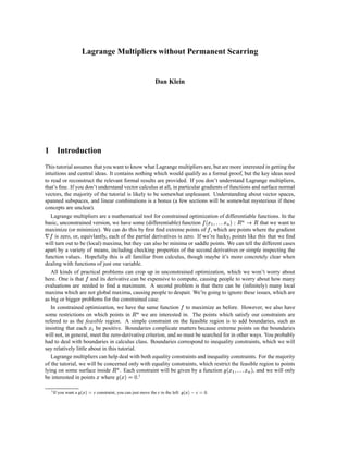
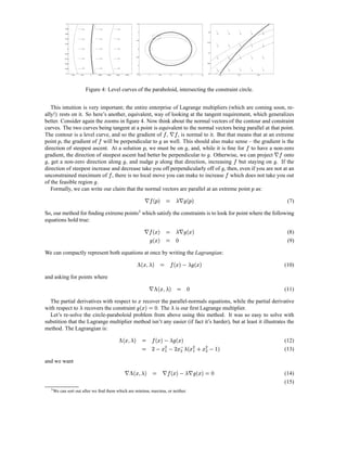
Figure 5: A spherical level curve of the function with two constraint planes, X S hP and s S hP .
directions that is free to vary. However, given the constraints, cannot make any local movement along
‘ ‘
vectors which have any component perpendicular to any constraint. Therefore, our condition should again be
¢ #
¡ ¡$ #
that ‘ , while not necessarily zero, is entirely contained in the subspace spanned by the normals. ‘
We can express this by the equation
“¦¤¢ #
0 £¡ t # %’
$ ¤—$
£¡
$ (28)
¢ #
¡ $ ’
Which asserts that be a linear combination of the normals, with weights .
‘
It turns out that tossing all the constraints into a single Lagrangian accomplishes this:
“—–¤¡ ”
0 ’§ £ 'ˆ$ ’ t '¢
£¡ $ £¡
$ P (29)
%•f'¡ ”
’§ £ $ ’
It should be clear that differentiating
q¦¤¡ $
2 0 £ with respect to and setting equal to zero recovers the th
$ £ u
constraint, , while differentiating with respect to the recovers the assertion that the gradient of
have no components which aren’t spanned by the constraints normals.
As an example of multiple constraints, consider figure ??. Imagine that is the distance from the origin.
Thus, the level surfaces of are concentric spheres with the gradient pointing straight out of the spheres. Let’s
0 0
say we want the minimum of subject to the constraints that and , shown as planes in the
X S hP s S hP
figure. Again imagine the spheres as expanding from the center, until it makes contact with the planes. The
#
unconstrained minimum is, of course, at the origin, where is zero. The sphere grows, and increases.
When the sphere’s radius reaches one, the sphere touches both planes individually. At the points of contact, the
gradient of is perpendicular to the touching plane. Those points would be solutions if that plane were the only
constraint. When the sphere reaches a radius of , it is touching both planes along their line of intersection.
I v
Note that the gradient is not zero at that point, nor is it perpendicular to either surface. However, it is parallel
to an (equal) combination of the two planes’ normal vectors, or, equivalently, it lies inside the plane spanned
t£
2 0
by those vectors (the plane , [not shown due to my lacking matlab skills]).
A good way to think about the effect of adding constraints is as follows. Before there are any constraints,
£
there are dimensions for to vary along when maximizing, and we want to find points where all dimensions
l l
have zero gradient. Every time we add a constraint, we restrict one dimension, so we have less freedom in
maximizing. However, that constraint also removes a dimension along which the gradient must be zero. So,
in the “nice” case, we should be able to add as many or few constraints (up to ) as we wish, and everything l
should work out.4
4 Inthe “not-nice” cases, all sorts of things can go wrong. Constraints may be unsatisfiable (e.g. s6
G @ and ws6
w @ , or subtler situations
can prevent the Lagrange multipliers from existing [more].

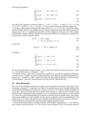
7. 3 The Lagrangian
'¡ $ $ ’ $ dr ¦¤¢xx%•f¤¡ ”
£ y £¡ 0 ’ § £ z {r yƒ£
|
The Lagrangian ’ is a function of
g| $ ’ z variables (remember that , plus
l z Ur
one for each of the ). Differentiating gives the corresponding equations, each set to zero, $ £ l
to solve. The equations from differentiating with respect to each
z l recovers our gradient conditions. The
$ %’ $
equations from differentiating with respect the recover the constraints . So the numbers give us some
confidence that we have the right number of equations to hope for point solutions.
It’s helpful to have an idea of what the Lagrangian actually means. There are two intuitions, described below.
3.1 The Lagrangian as an Encoding
First, we can look at the Lagrangian as an encoding of the problem. This view is easy to understand (but doesn’t $
really get us anywhere). Whenever the constraints are satisfied, the are zero, and so at these point, regarless
$ ’ '¢3}%•f¤¡ ”
£¡ 0 ’§ £
of the value of the multipliers, . This is a good fact to keep in mind.
£ You could imagine using the Lagrangian to do constrained maximization in the following way. You move
’
around looking for a maximum value of . However, you have no control over , which gets set in the
£ ƒnz
‚ ”
worst way possible for you. Therefore, when you choose ,
£ is chosen to minimize . Formally, the
 €~ 
problem is to find the which gives
…F
0 „ ˆ%•f¤¡ ” ŽŒ¤¡ ¨ˆ†
’ § £ ‹ † ‰ ‡
 Š (30)
'¢m`—–¤¡ ”
£¡ 0 ’§ £ ’
Now remember that if your x happens to satisfy the constraints,
£ , regardless of what is.
’‘'ˆ$
2 0 £ ¡ $ ’ —f'¡ ”
’§ £
However, if does not satisfy the constraints, some
%•f'¡ ”  Ž‘†
’§ £ ‹ . But then, can be fiddled to make
„
as small as desired, and will be . So will be the maximum value of subject to the
“ eP
constraints.
3.2 Reversing the Scope
The problem with the above view of the Lagrangian is that it really doesn’t accomplish anything beyond en-
coding the constraints and handing us back the same problem we started with: find the maximum value of ,
£ ŽŒ†
‹ ¨ˆ†
‰‡
ignoring the values of which are not in the feasible region. More usefully, we can switch the and
from the previous section, and the result still holds:
„ 0 ˆ%•f¤¡ ” ¨ˆ¤¡ ŽŒ†
’ § £ ‰ ‡ † ‹
Š  (31)
This is part of the full Kuhn-Tucker theorem (cite), which we aren’t going to prove rigorously. However, the
intuition behind why it’s true is important. Before we examine why this reversal should work, let’s see what it
accomplishes if it’s true.
We originally had a constrained optimization problem. We would very much like for it to become an uncon-$ ’ —f'¡ ”
’§ £ £
strained optimization problem. Once we fix the values of the multipliers, becomes a function of
alone. We might be able to maximize that function (it’s unconstrained!) relatively easily. If so, we would get a
’ €¡ „ £
’ €¡ „ £
’
solution for each , call it
’ . But then we can do an unconstrained minimization of over the space
of . We would then have our solution.
£ '¡ „ ’
£ £
It might not be clear why that’s any different that fixing and finding a minimizing value
'¡ „ ’ %‡¡ „ £
£ ’ for each .
It’s different in two ways. First, unlike , would not be continuous. (Remember that it’s negative
£ '¢
£¡
infinity almost everywhere and jumps to for which satisfy the constraints.) Second, it is often the case
%‡¡ „ £
’ ¦¤¡ „ ’
£
that we can find a closed-form solution to while we have nothing useful to say about . This is also
a general instance of switching to a dual problem when a primal problem is unpleasant in some way. [cites]
3.3 Duality
Let’s say we’re convinced that it would be a good thing if
“—–¤¡ ” 7Œ¤¡ (Œ†
0 ’ § £ ‹ † ‰ ‡ ˆ%•f'¡ ” ¨ˆ¤¡ 7Œ†
’ § £ ‰ ‡ † ‹
 Š Š  (32)

8. 10
5
0
−5
−10
−15
−20
−25
−30
−35
4
2 4
2
0
0
−2
−2
−4 −4
R %£ £ 2 30
Figure 6: The Lagrangian of the paraboloid P VI with the constraint S TP .
Now, we’ll argue why this is true, examples first, intuition second, formal proof elsewhere. Recall the no-
1¦¤¢
0 £¡ R %£ £ 2 t0
brainer problem: maximize subject to P VI . Let’s form the Lagrangian. S TP
“—–¤¡ ”
0 ’§ £ R £ ¤–’
£¡
P VI P S TP (33)
0 t£ ”
This surface is plotted in figure ??. The straight dark line is the value of at
’ . At that value, the ” 0 £ ¡S 0 ’ § £ ‚ 
c'¢–V—–¤¡ •Hz £
constraint is satisfied and so, as promised, has no effect on and
'¡ „ ’
£ 0 £ ™¦¤¡ „ ’
0 £ . At each , S
%’‡¡ „ £U0£ ”   ™”
’ be , except for
” “ eP where S . The curving dark line is the value of at
S %‡¡ „ £
’ 0 i£ for all
n•§
0 ’ 0 i
. The minimum value along this
¤¢
£¡ line is at , where , which is the maximum (and
S I S
only) value of among the point(s) satisfying the constraint.
3.4 A sort-of proof of sort-of the Kuhn-Tucker thereom
The Lagrangian is hard to plot when . However, let’s consider what happens in the environment of a point
3ƒl
S —
‘ which satisfies the constraints, and which is a local maximum among the points satisfying the constraints.
a} $
2 0 ¡ %’•§f¤¡ ”
£ ¢ #
¡ $ %’
Since each
¢ #¡ , the derivatives of
‘ with respect to each are zero. may not be zero. But
¡—$ # ‘
if ‘ has any component which is not in the space spanned by the constraint normals , then we can
‘ ¢ ¡
nudge in a direction inside the allowed region, increasing
‘ ¢ #. Since is a local minimum inside that region,
¡ $ #
¡ ‘ ‘
that isn’t possible. So is in the space spanned by the constraint normals
‘ , and can therefore be ‘ ¡ $ # $ ’ $ y Y ¢ #
0 ¡
written as a (unique) linear combination of these normals. Let
2U™ ¡ $ # $ ’ $ y ¢ #
0 ¡ be that combination. ‘ ‘
Then clearly .
¡ $ # ˜$%’ $ y ¢ # ‘ ’ %’ P ‘
¡ ˜
Now consider a vector near .
ˆ$ # ‘ %’ $ y ¢P # ‘ 0}™%—§ ¡ ” #
¡ ˜ ¡ ˜ ’ cannot still be zero, because the linear combination
’ ˜ %’
weights are unique. But‘ $ P š‘%’—§ ¡ ” # ‘
˜ is non-zero. Thus, fixing and allowing to ” ‘
vary, there is some direction (either ‘ or the reverse direction where we could nudge to increase .
€¡ „ £ f’
’ ¡ ‘
Therefore, at , is at a local minimum. ‘
’
Another way to remember this intuitively is that is probably not zero, and, if we set it to zero (a huge
” '¢mY›ˆf'¡ ”
£¡ 0 2§ £
nudge), , and so the maximum of is the unconstrained maximum of , which can only be
¢ ¡
larger than . ‘ £
Let’s look another more example. Recall the paraboloid (figure 5) with the constraint that and sum to one.
0y § ux –¤¡ ¡ 0 § £ ’ X
The maximum value occured at
i¨kf g0n’
h 2 ¨jS (‰I
ih ih , where
X ’ . The value was . Figure 7 shows ” ¨h gP
i f
what happens when we nudge up and down slightly. At
, the Lagrangian is just the original surface 0 w’
. Its maximum value (2) is at the origin (which obviously doesn’t satisfy the constraint). At
¡ q0 § , the (h gP
i f
maximum value of the Lagrangian is at , (which does satisfy the constraints). The gradient of
‘ ¨¨S (‰I
ih ih
is not zero, but it is perpendicular to the constraint line, so is a local maximum along that line. Another way
‘
of thinking of this is that the gradient of (the top arrow field) is balanced at that point by the scaled gradient
of the constraint (the second arrow field down). We can see the effect by adding these two fields, which forms ’ ’
the gradient of the Lagrangian (third arrow field). This gradient is zero at with the right . If we nudge up
© D2 r ‘ # ’
to ¨kgP
ih f , then suddenly the gradient of is no longer completely cancelled out by
S , and so we can

9. lambda = 0 lambda = −1.6667 lambda = −1.3333 lambda = −1
2 2 2 2
0 0 0 0
−2 −2 −2 −2
−2 0 2 −2 0 2 −2 0 2 −2 0 2
2 2 2 2
0 0 0 0
−2 −2 −2 −2
−2 0 2 −2 0 2 −2 0 2 −2 0 2
2 2 2 2
0 0 0 0
−2 −2 −2 −2
−2 0 2 −2 0 2 −2 0 2 −2 0 2
2 2 2 2
0 0 0 0
−2 −2 −2 −2
−2 0 2 −2 0 2 −2 0 2 −2 0 2
R %£ R r £ 2 t0
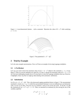
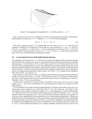
Figure 7: Lagrangian surfaces for the paraboloid P VI (P
XI with the constraint vEX
S P .
’ © D2
increase the lagrangian by nudging toward the origin. Similarly, if we nudge down to
‘ , then the g(h gP
P i f S
gradient of is over-cancelled and we can increase the Lagrangian by nudging away from the origin. ‘
3.5 What do the multipliers mean?
A useful aspect of the Lagrange multiplier method is that the values of the multipliers at solution points often
$ ’ ”
has some significance. Mathematically, a multiplier is the value of the partial derivative of with respect to
$
the constraint . So it is the rate at which we could increase the Lagrangian if we were to raise the target of that
¢a™—§ ¡ ”
¡ 0 ’
constraint (from zero). But remember that at solution points , . Therefore, the rate of increase
‘ ‘ ‘
of the Lagrangian with respect to that constraint is also the rate of increase of the maximum constrained value
of with respect to that constraint.
$ $ ’
In economics, when is a profit function and the are constraints on resource amounts,
would be the
amount (possibly negative!) by which profit would rise if one were allowed one more unit of resource . This u
rate is called the shadow price of , which is interpreted as the amount it would be worth to relax that constraint
u
upwards (by RD, mining, bribery, or whatever means).
[Physics example?]
4 A bigger example than you probably wanted
This section contains a big example of using the Lagrange multiplier method in practice, as well as another
case where the multipliers have an interesting interpretation.

10. 1
0.8
0.6
0.4
0.2
0
0 0
0.2 0.2
0.4 0.4
0.6 0.6
0.8 0.8
1 1
r £ r 0
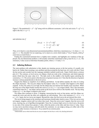
Figure 8: The simplex X s S .
4.1 Maximum Entropy Models
5 Extensions
5.1 Inequality Constraints
The Lagrange multiplier method also covers the case of inequality constraints. Constraints of this form are
qˆ¤¡
2  £ £ '¡
£
written 3™'œ ¡
2 0 £ . The key observation about inequality constraints work is that, at any given , a
¦¤¡
£ 2 has œ
either
œ or
2 0 œ £
’V'¡ , which are qualitatively very different. The two possibilities are shown in figure ??.
— £ £
If œ then is said to be active at , otherwise it is inactive. If is active at , then is a lot like an
œ £ £œ
¦¤¡¢ # œ
equality constraint; it allows to be maximum if the gradient of , , is either zero or pointing towards
negative values of (which violate the constraint). However, if the gradient is pointing towards positive values
œ
of , then there is no reason that we cannot move in that direction. Recall that we used to write
œ
# t™¦¤¢ #
’ 0 £¡ '¡
£
(34)
£ '¢ #
£¡
for a (single) equality constraint. The interpretation was that, if is a solution, must be entirely in the
# '¡
£ '¡
£
direction of the normal to , . For inequality constraints, we write
# t™¦¤¢ #
ž 0 £¡ ¦¤¡
£
œ (35)
¦¤¢ #
£¡ # ¤¡
£
but, if x is a maximum, then if is non-zero, it not only has to be parallel , but it must actually
point in the opposite sense along that direction (i.e., out of the feasible side and towards the forbidden side). We
can actually enforce this very simply, by restricting the multiplier to be negative (or zero). Positive mutlipliers
¦¤¡
£
mean that the direction of increasing is in the same direction as increasing – but points in that situation
œ
certainly aren’t solutions, as we want to increase and we are allowed to increase .
2 '¡ £
£ œ ž
If is inactive at (
œ ), then we want to be even stricter about what values of are acceptable from
ž — œ £
a solution. In fact, in this case, must be zero at . (Intuitively, if is inactive, then nothing should change at
£ œ
if we drop ). [better explanation]
œ
In summary, for inequality constraints, we add them to the Lagrangian just as if they were equality con-
tWž
2 Ÿ ¦¤¡
£ ž
straints, except that we require that and that, if is not zero, then is. The situation that one or the œ
other can be non-zero, but not both, is referred to as complementary slackness. This situation can be compactly
U}¤¡ ž
2 0 £
written as œ . Bundling it all up, complete with multiple constraints, we get the general Lagrangian:
¦¤¡
£ ž (t ¦¤—$ %’ t ¦¤¢3™ff—–¤¡ ”
£¡ $ £¡ 0 ž§ ’§ £
œ P $ P (36)
£
The Kuhn-Tucker theorem (or our intuitive arguments) tell us that if a point
$ $ is a maximum of subject to
the constraints and , then:
œ
“ff—–¤¡ ” #
0 ž§ ’§ £ '¢ #
£¡ t # ’
$ 'ˆ$
£¡ # ž (t
3™'¡
2 0 £
P $ P œ (37)

11. $ § ¡
ž Ÿ 2
u (38)
0“'¡
£ ž t 2
œ (39)
The second condition takes care of the restriction on active inequalities. The third condition is a somewhat
$ ž ¦¤¡ $
£
cryptic way of insisting that for each , either is zero or
u œ is zero.
Now is probably a good time to point out that there is more to the Kuhn-Tucker theorem than the above
statement. The above conditions are called the first-order conditions. All (local) maxima will satisfy them. The
theorem also gives second order conditions on the second derivative (Hessian) matrices which distinguish local
maxima from other situations which can trigger “false alarms” with the first-order conditions. However, in
many situations, one knows in advance that the solution will be a maximum (such as in the maximum entropy
example).
Caveat about globals?
6 Conclusion
This tutorial only introduces the basic concepts of the Langrange multiplier methods. If you are interested,
there are many detailed texts on the subject [cites]. The goal of this tutorial was to supply some intuition
behind the central ideas so that other, more comprehensive and formal sources become more accessible.
Feedback requested!