Downloaded 313 times
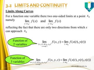
![rahimahj@ump.edu.my
0)G(ifmadebecansconclusionNo(iv)
0)G(ifpointsaddleais)),(,,((iii)
0),(and0)G(ifminimumlocalais),((ii)
0),(and0)G(ifmaximumlocalais),((i)
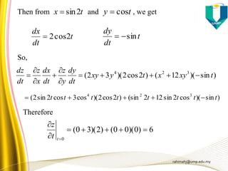
Then
)],([),(),(
),(),(
),(),(
)G(
LetR.inpointcriticalais
b)(a,andRregionaonsderivativepartialsecondcontinuous
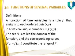
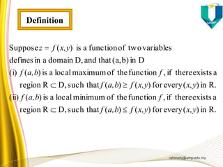
hasthatvariablestwooffunctionais)(thatSuppose
2
a,b
a,bbafba
bafa,bbaf
bafa,bbaf
bafbafbaf
bafbaf
bafbaf
a,b
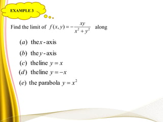
x,yf
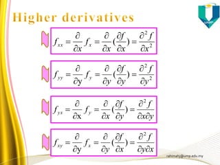
xx
xx
xyyyxx
yyxy
xyxx
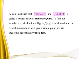
TestDerivativeSecond:Theorem](https://image.slidesharecdn.com/chapter3partialderivatives-150105021210-conversion-gate02/85/Applied-Calculus-Chapter-3-partial-derivatives-58-320.jpg)


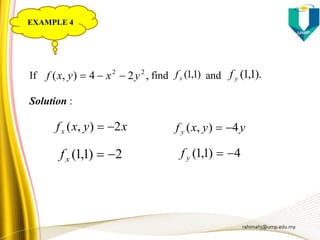
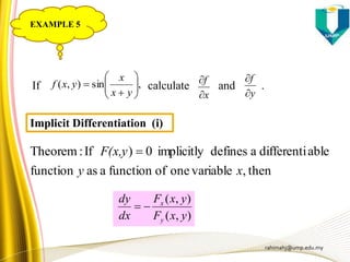
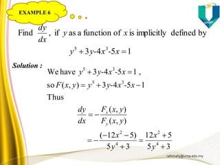
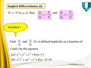
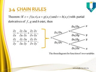
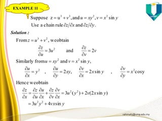
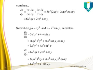
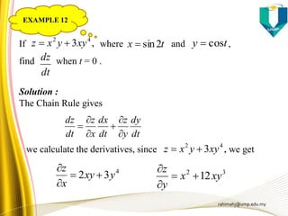
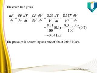
1) The document discusses partial derivatives, which involve differentiating functions of two or more variables with respect to one variable while holding the others constant. It provides examples of computing first and second partial derivatives. 2) Implicit differentiation is introduced as a way to find partial derivatives of functions defined implicitly rather than explicitly. The chain rule is also discussed. 3) Methods are presented for finding partial derivatives of functions of two or three variables, including using implicit differentiation and the chain rule. Examples are provided to illustrate these concepts.


