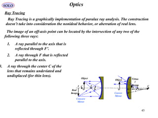
Downloaded 191 times
![10
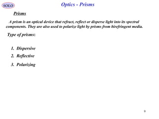
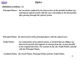
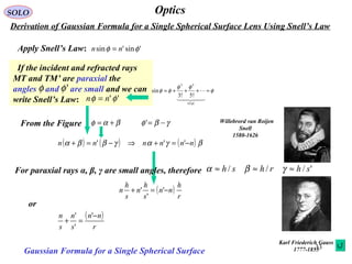
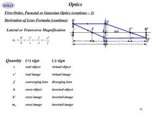
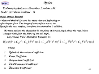
OpticsSOLO
Dispersive Prisms
( ) ( )2211 itti
θθθθδ −+−=
21 it
θθα +=
αθθδ −+= 21 ti
202
sinsin ti
nn θθ =Snell’s Law
10
≈n
( ) ( )[ ]1
1
2
1
2
sinsinsinsin tit
nn θαθθ −== −−
( )[ ] ( )[ ]11
21
11
1
2 sincossin1sinsinsincoscossinsin ttttt nn θαθαθαθαθ −−=−= −−
Snell’s Law 110
sinsin ti
nn θθ =
11
sin
1
sin it
n
θθ =
( )[ ]1
2/1
1
221
2 sincossinsinsin iit n θαθαθ −−= −
( )[ ] αθαθαθδ −−−+= −
1
2/1
1
221
1
sincossinsinsin iii
n
The ray deviation angle is
10
≈n](https://image.slidesharecdn.com/lens-141229120650-conversion-gate01/85/Lens-10-320.jpg)
![11
OpticsSOLO
Prisms
( )[ ] αθαθαθδ −−−+= −
1
2/1
1
221
1
sincossinsinsin iii
n](https://image.slidesharecdn.com/lens-141229120650-conversion-gate01/85/Lens-11-320.jpg)
![12
OpticsSOLO
Prisms
( )[ ] αθαθαθδ −−−+= −
1
2/1
1
221
1
sincossinsinsin iii
n
αθθδ −+= 21 ti
Let find the angle θi1 for which the deviation angle δ is minimal; i.e. δm.
This happens when
01
0
11
2
1
=−+=
ii
t
i d
d
d
d
d
d
θ
α
θ
θ
θ
δ
Taking the differentials
of Snell’s Law equations
22
sinsin ti
n θθ =
11
sinsin ti
n θθ =
2222
coscos iitt
dnd θθθθ =
1111
coscos ttii
dnd θθθθ =
Dividing the equations
1
2
1
2
1
1
2
1
2
1
cos
cos
cos
cos
−−
=
i
t
i
t
t
i
t
i
d
d
d
d
θ
θ
θ
θ
θ
θ
θ
θ
2
22
1
22
2
2
2
2
1
2
2
2
1
2
2
2
1
2
sin
sin
/sin1
/sin1
sin1
sin1
sin1
sin1
t
i
t
i
i
t
t
i
n
n
n
n
θ
θ
θ
θ
θ
θ
θ
θ
−
−
=
−
−
=
−
−
=
−
−
1
1
2
−=
i
t
d
d
θ
θ
21 it
θθα +=
1
2
1
−=
i
t
d
d
θ
θ
2
2
1
2
2
2
1
2
cos
cos
cos
cos
i
t
t
i
θ
θ
θ
θ
= 21 ti
θθ =
1≠n](https://image.slidesharecdn.com/lens-141229120650-conversion-gate01/85/Lens-12-320.jpg)
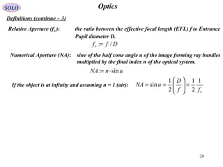
![13
OpticsSOLO
Prisms
( )[ ] αθαθαθδ −−−+= −
1
2/1
1
221
1 sincossinsinsin iii n
We found that if the angle θi1 = θt2 the deviation angle δ is minimal; i.e. δm.
Using the Snell’s Law
equations
22
sinsin ti
n θθ =
11
sinsin ti
n θθ = 21 ti
θθ =
21 it
θθ =
This means that the ray for which the deviation angle δ is minimum passes through
the prism parallel to it’s base.
Find the angle θi1 for
which the deviation
angle δ is minimal; i.e.
δm (continue – 1(.](https://image.slidesharecdn.com/lens-141229120650-conversion-gate01/85/Lens-13-320.jpg)
![14
OpticsSOLO
Prisms
( )[ ] αθαθαθδ −−−+= −
1
2/1
1
221
1 sincossinsinsin iii n
Using the Snell’s Law 11
sinsin ti
n θθ =
21 it
θθ =
This equation is used for determining the refractive index of transparent substances.
21 it
θθα +=
αθθδ −+= 21 ti
21 ti
θθ =
mδδ =
2/1 αθ =t
αθδ −= 12 im
( ) 2/1 αδθ += mi
( )[ ]
2/sin
2/sin
α
αδ +
= m
n
Find the angle θi1 for
which the deviation
angle δ is minimal; i.e.
δm (continue – 2(.](https://image.slidesharecdn.com/lens-141229120650-conversion-gate01/85/Lens-14-320.jpg)
![15
OpticsSOLO
Prisms
The refractive index of transparent substances varies with the wavelength λ.
( )[ ]{ } αθαθλαθδ −−−+= −
1
2/1
1
221
1
sincossinsinsin iii
n](https://image.slidesharecdn.com/lens-141229120650-conversion-gate01/85/Lens-15-320.jpg)
![16
OpticsSOLO
http://physics.nad.ru/Physics/English/index.htm
Prisms
Color λ0 (nm( υ [THz]
Red
Orange
Yellow
Green
Blue
Violet
780 - 622
622 - 597
597 - 577
577 - 492
492 - 455
455 - 390
384 – 482
482 – 503
503 – 520
520 – 610
610 – 659
659 - 769
1 nm = 10-9
m, 1 THz = 1012
Hz
( )[ ]{ } αθαθλαθδ −−−+= −
1
2/1
1
221
1
sincossinsinsin iii
n
In 1672 Newton wrote “A New Theory about Light and Colors” in which he said that
the white light consisted of a mixture of various colors and the diffraction was color
dependent.
Isaac Newton
1542 - 1727](https://image.slidesharecdn.com/lens-141229120650-conversion-gate01/85/Lens-16-320.jpg)
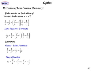
![32
OpticsSOLO
Derivation of Gaussian Formula for a Single Spherical Surface Lens Using Fermat’s Principle
Karl Friederich Gauss
1777-1855
The optical path connecting points M, T, M’ is
''lnlnpathOptical ⋅+⋅=
Applying cosine theorem in triangles MTC and M’TC
we obtain:
( ) ( )[ ] 2/122
cos2 βRsRRsRl +−++=
( ) ( )[ ] 2/122
cos'2'' βRsRRsRl −+−+=
( ) ( )[ ] ( ) ( )[ ] 2/122
2/122
cos'2''cos2 ββ RsRRsRnRsRRsRnpathOptical −+−+⋅++−++⋅=
Therefore
According to Fermat’s Principle when the point T
moves on the spherical surface we must have ( ) 0=
βd
pathOpticald
( ) ( ) ( ) 0
'
sin''sin
=
−⋅
−
+⋅
=
l
RsRn
l
RsRn
d
pathOpticald ββ
β
from which we obtain
⋅
−
⋅
=+
l
sn
l
sn
Rl
n
l
n
'
''1
'
'
For small α and β we have ''& slsl ≈≈
and we obtain
R
nn
s
n
s
n −
=+
'
'
'
Gaussian Formula for a Single Spherical Surface](https://image.slidesharecdn.com/lens-141229120650-conversion-gate01/85/Lens-32-320.jpg)
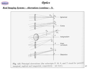
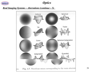
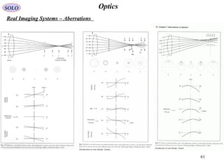
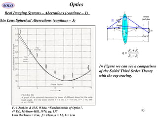
![62
OpticsSOLO
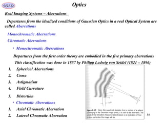
Real Imaging Systems – Aberrations (continue – 1)
Seidel Aberrations
Consider a spherical surface of radius R, with an object P0 and the image P0’ on the
Optical Axis.
The Chief Ray is P0 V0 P0’ and a
General Ray P0 Q P0’.
The Wave Aberration is defined as
the difference in the optical path
lengths between a General Ray and
the Chief Ray.
( ) [ ] [ ] ( ) ( )snsnQPnQPnPVPQPPrW +−+=−= '''''' 00000000
On-Axis Point Object
The aperture stop AS, entrance pupil EnP,
and exit pupil ExP are located at the
refracting surface.](https://image.slidesharecdn.com/lens-141229120650-conversion-gate01/85/Lens-62-320.jpg)
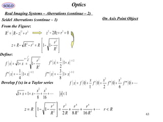
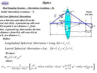
![64
OpticsSOLO
Real Imaging Systems – Aberrations (continue – 3)
Seidel Aberrations (continue – 2)
From the Figure:
( )[ ] [ ]
( )[ ] ( ) 2/1
2
2/12
2
2/12222/122
0
212
2
22
−
+=+−=
++−=+−=
−=
z
s
sR
sszsR
rsszzrszQP
rzRz
( ) ( )
+
−
−
−
+−≈
<++−+=+
2
4
2
2
1
168
11
2
1
1
32
z
s
sR
z
s
sR
s
x
xx
xx
( ) ( )
+
+
−
−
+
−
+−=
+≈
2
3
42
4
2
3
42
2
82
822
1
82
1
3
42
R
r
R
r
s
sR
R
r
R
r
s
sR
s
R
r
R
r
z
( )[ ] +
−+
−+
−+−≈+−= 4
2
2
22/122
0
11
8
111
8
111
2
1
r
sRssRR
r
sR
srszQP
( )[ ] +
−+
−+
−+≈+−= 4
2
2
22/122
0
1
'
1
'8
11
'
1
8
11
'
1
2
1
''' r
RssRsR
r
Rs
srzsPQ
In the same way:
On Axis Point Object](https://image.slidesharecdn.com/lens-141229120650-conversion-gate01/85/Lens-64-320.jpg)
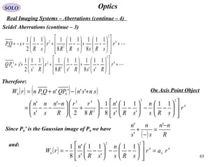
![67
OpticsSOLO
Real Imaging Systems – Aberrations (continue – 6)
Seidel Aberrations (continue – 5)
Off-Axis Point Object
The Wave Aberration is defined as the difference
n the optical path lengths between the General
Ray and the Undeviated Ray.
( ) [ ] [ ]
[ ] [ ]{ } [ ] [ ]{ }
( )4
0
4
0 ''''
''
VVVQa
PVPPPVPVPPQP
PVPPQPQW
S −=
−−−=
−=
For the approximately similar triangles VV0C and CP0’P’ we have:
CP
CV
PP
VV
''' 0
0
0
0
≈ ''
'
''
'
0
0
0
0 hbh
Rs
R
PP
CP
CV
VV =
−
=≈
Rs
R
b
−
=
'
:
−−
−−=
22
11
'
11
'
'
8
1
sRs
n
sRs
n
aS](https://image.slidesharecdn.com/lens-141229120650-conversion-gate01/85/Lens-67-320.jpg)
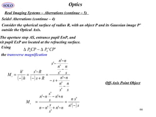
![68
OpticsSOLO
Real Imaging Systems – Aberrations (continue – 7)
Seidel Aberrations (continue – 6)
Off-Axis Point Object
Wave Aberration.
( ) [ ] [ ] ( )4
0
4
'' VVVQaPVPPQPQW S −=−=
Define the polar coordinate (r,θ) of the projection of Q in the plane of exit pupil, with
V0 at the origin.
θθ cos'2'cos2 222
0
2
0
2
2
hbrhbrVVrVVrVQ ++=++=
'0 hbVV =
( ) [ ] [ ] ( )
( )[ ]442222
4
0
4
'cos'2'
''
hbhbrhbra
VVVQaPVPPQPQW
S
S
−++=
−=−=
θ
( ) ( )θθθθ cos'4'2cos'4cos'4';, 33222222234
rhbrhbrhbrhbrahrW S ++++=](https://image.slidesharecdn.com/lens-141229120650-conversion-gate01/85/Lens-68-320.jpg)
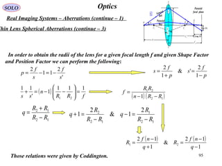
![74
OpticsSOLO
Real Imaging Systems – Aberrations (continue – 1)
1. Spherical Aberrations
( )
( ) ( )';','''
';,
222
4
hyxWyxC
rChrW
SpSp
SpSp
=+=
=θ
( ) '
'
'
4
'
';','
'
'
' 2
xrC
n
L
x
hyxW
n
L
x Sp
=
∂
=∆
( ) '
'
'
4
'
';','
'
'
' 2
yrC
n
L
y
hyxW
n
L
y Sp
=
∂
=∆
To Update
( ) ( )[ ] 32/122
'
'
4'' rC
n
L
yxr Sp=∆+∆=∆
Consider only the Spherical Wave Aberration Function
The Spherical Wave Aberration is a
Circle in the Image Plane](https://image.slidesharecdn.com/lens-141229120650-conversion-gate01/85/Lens-74-320.jpg)
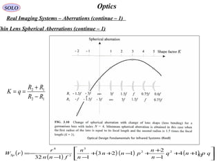
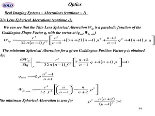
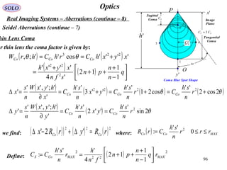
![86
OpticsSOLO
Real Imaging Systems – Aberrations (continue – 8)
Seidel Aberrations (continue – 7)
hin Lens Aberrations
( ) 2222234
'cos'cos'';, rhCrhCrhCrChrW FCAsCoSp +++= θθθ
ven a thin lens formed by two
faces with radiuses r1 and r2
h centers C1 and C2. PP0 is
object, P”P”0 is the Gaussian
ge formed by the first surface,
’0 is the image of virtual object
”0 of the second surface.
( )
( ) ( ) ( )
++
−
+
+−++
−−
−= qpnq
n
n
pnn
n
n
fnn
CSp 14
1
2
123
1132
1 22
3
3
( )
−
+
++= q
n
n
pn
sfn
CCo
1
1
12
'4
1
2
( )2
'2/1 sfCAs −=
( ) ( )2
'4/1 sfnnCFC +−=
where:
f
s
OA
C11
r
F”
F
''f
''s
2
r
1=n
n
h
"h
D
0P
P
0'P
0"P
"P
'P
'h
's
CR
AS
EnP
ExP
r
( )θ,rQ
OC2
1=n
( ) [ ] [ ]0000 '', OPPQPPrW −=θ
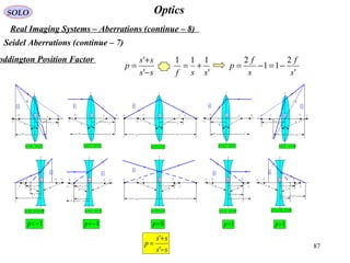
Coddington shape factor:
Coddington position factor: ss
ss
p
−
+
=
'
'
12
12
rr
rr
q
−
+
=
From:
we find:](https://image.slidesharecdn.com/lens-141229120650-conversion-gate01/85/Lens-85-320.jpg)
![115
SOLO
References
[1] M. Born, E. Wolf, “Principle of Optics – Electromagnetic Theory of Propagation,
Interference and Diffraction of Light”, 6th
Ed., Pergamon Press, 1980,
[2] C.C. Davis, “Laser and Electro-Optics”, Cambridge University Press, 1996,
OPTICS](https://image.slidesharecdn.com/lens-141229120650-conversion-gate01/85/Lens-114-320.jpg)
![116
SOLO
References
Foundation of Geometrical Optics
[3] E.Hecht, A. Zajac, “Optics ”, 3th
Ed., Addison Wesley Publishing Company, 1997,
[4] M.V. Klein, T.E. Furtak, “Optics ”, 2nd
Ed., John Wiley & Sons, 1986](https://image.slidesharecdn.com/lens-141229120650-conversion-gate01/85/Lens-115-320.jpg)


The document provides a comprehensive overview of geometrical optics, including foundational principles such as Fermat's principle, the laws of reflection and refraction, and various types of optical devices like lenses and prisms. It elaborates on the mathematical relationships governing ray behavior as light interacts with different media and covers applications of these principles in devices such as dispersing and reflecting prisms. Key definitions related to optical systems, including focal points and stops, are also explained to illustrate how they influence image formation.


