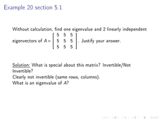
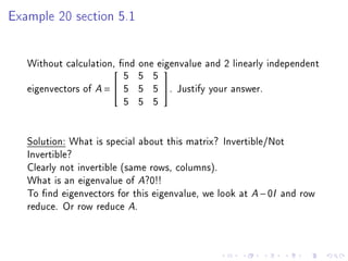
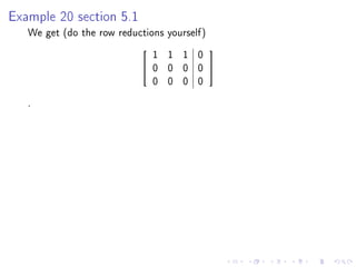
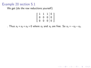
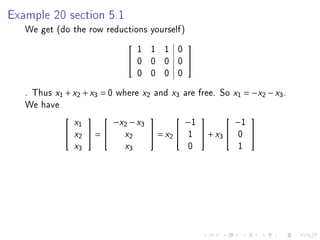
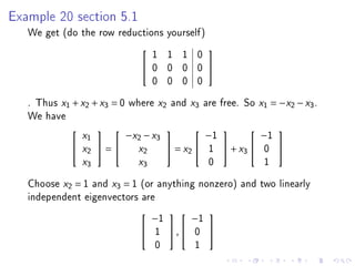
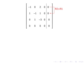
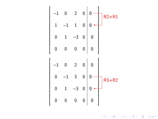
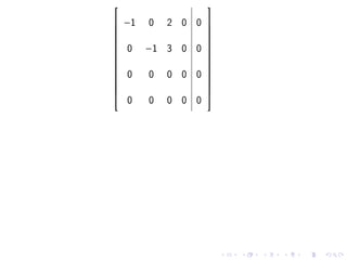
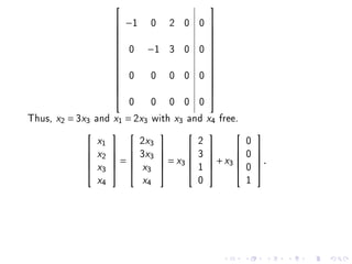
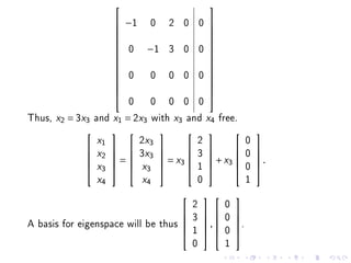
1. The matrix is not invertible as it has repeated rows. 2. The eigenvalue is 0 since a matrix is not invertible if it has 0 as an eigenvalue. 3. The eigenvectors corresponding to 0 can be found by reducing the matrix A - 0I to row echelon form. This gives the equation x1 + x2 + x3 = 0 with x2 and x3 as free variables, so two linearly independent eigenvectors are (1, -1, 0) and (1, 0, -1).

1. Announcements
Quiz 3 after lecture.
Grades will be updated online (including quiz 3 grades) over
the weekend. Please let me know if you spot any mistakes.
Exam 2 will be on Feb 25 Thurs in class. Details later.
Make-up exams will be given only if there is an excused
absence from the Dean of Students or a Doctor's note about
sudden serious illness. No exceptions on this. Travel
plans/broken alarm clock are unacceptable excuses.

2. Last Class...
Denition
An eigenvector of an n × n matrix A is a NON-ZERO vector x
such that Ax = λx for some scalar λ.
A scalar λ is called an eigenvalue of A if there is a nontrivial (or
nonzero) solution x to Ax = λx; such an x is called an eigenvector
corresponding to λ.

3. Triangular Matrices
Theorem
The eigenvalues of a triangular matrix are the entries on its main
diagonal.

4. Triangular Matrices
Example
1. Let
5 1 9
 
A = 0 2 3 
0 0 6
The eigenvalues of A are 5, 2 and 6.

5. Triangular Matrices
Example
1. Let
5 1 9
 
A = 0 2 3 
0 0 6
The eigenvalues of A are 5, 2 and 6.
2. Let
4 1 9
 
A= 0 0 3 
0 0 6
The eigenvalues of A are 4, 0 and 6.

6. Zero Eigenvalue??
Zero eigenvalue means
1. The equation Ax = 0x has a nontrivial or nonzero solution

7. Zero Eigenvalue??
Zero eigenvalue means
1. The equation Ax = 0x has a nontrivial or nonzero solution
2. This means Ax = 0 has a nontrivial solution.

8. Zero Eigenvalue??
Zero eigenvalue means
1. The equation Ax = 0x has a nontrivial or nonzero solution
2. This means Ax = 0 has a nontrivial solution.
3. This means A is not invertible (or det A = 0) (by invertible
matrix theorem)

9. Zero Eigenvalue??
Zero eigenvalue means
1. The equation Ax = 0x has a nontrivial or nonzero solution
2. This means Ax = 0 has a nontrivial solution.
3. This means A is not invertible (or det A = 0) (by invertible
matrix theorem)
Zero is an eigenvalue of A if and only if A is not invertible

10. Important
If λ is an eigenvalue of a square matrix A, prove that λ2 is an
eigenvalue of A2 .
For any problem of this type, start with the equation that denes
eigenvalue and take it from there.

11. Important
If λ is an eigenvalue of a square matrix A, prove that λ2 is an
eigenvalue of A2 .
For any problem of this type, start with the equation that denes
eigenvalue and take it from there.
Solution: If λ is an eigenvalue of a square matrix A, we have
Ax = λx.

12. Important
If λ is an eigenvalue of a square matrix A, prove that λ2 is an
eigenvalue of A2 .
For any problem of this type, start with the equation that denes
eigenvalue and take it from there.
Solution: If λ is an eigenvalue of a square matrix A, we have
Ax = λx.
Multiply both sides by A. We get A2 x = A(λx).

13. Important
If λ is an eigenvalue of a square matrix A, prove that λ2 is an
eigenvalue of A2 .
For any problem of this type, start with the equation that denes
eigenvalue and take it from there.
Solution: If λ is an eigenvalue of a square matrix A, we have
Ax = λx.
Multiply both sides by A. We get A2 x = A(λx).
This is same as writing A2 x = λ (Ax) since λ is a scalar.

14. Important
If λ is an eigenvalue of a square matrix A, prove that λ2 is an
eigenvalue of A2 .
For any problem of this type, start with the equation that denes
eigenvalue and take it from there.
Solution: If λ is an eigenvalue of a square matrix A, we have
Ax = λx.
Multiply both sides by A. We get A2 x = A(λx).
This is same as writing A2 x = λ (Ax) since λ is a scalar.
Again Ax = λx. So, A2 x = λ (λx) = λ2 x.

15. Important
If λ is an eigenvalue of a square matrix A, prove that λ2 is an
eigenvalue of A2 .
For any problem of this type, start with the equation that denes
eigenvalue and take it from there.
Solution: If λ is an eigenvalue of a square matrix A, we have
Ax = λx.
Multiply both sides by A. We get A2 x = A(λx).
This is same as writing A2 x = λ (Ax) since λ is a scalar.
Again Ax = λx. So, A2 x = λ (λx) = λ2 x. This equation means that
λ2 is an eigenvalue of A2 .

16. Important, see prob 25 sec 5.1
If λ is an eigenvalue of an invertible matrix A, prove that λ−1 is an
eigenvalue of A−1 .

17. Important, see prob 25 sec 5.1
If λ is an eigenvalue of an invertible matrix A, prove that λ−1 is an
eigenvalue of A−1 .
Solution: If λ is an eigenvalue of a square matrix A, we have
Ax = λx.

18. Important, see prob 25 sec 5.1
If λ is an eigenvalue of an invertible matrix A, prove that λ−1 is an
eigenvalue of A−1 .
Solution: If λ is an eigenvalue of a square matrix A, we have
Ax = λx.
Since A is invertible, multiply both sides by A−1 . We get
−1
A A x = A−1 (λx)
I

19. Important, see prob 25 sec 5.1
If λ is an eigenvalue of an invertible matrix A, prove that λ−1 is an
eigenvalue of A−1 .
Solution: If λ is an eigenvalue of a square matrix A, we have
Ax = λx.
Since A is invertible, multiply both sides by A−1 . We get
−1
A A x = A−1 (λx) =⇒ A−1 (λx) = x
I

20. Important, see prob 25 sec 5.1
If λ is an eigenvalue of an invertible matrix A, prove that λ−1 is an
eigenvalue of A−1 .
Solution: If λ is an eigenvalue of a square matrix A, we have
Ax = λx.
Since A is invertible, multiply both sides by A−1 . We get
−1
A A x = A−1 (λx) =⇒ A−1 (λx) = x
I
This is same as writing λ(A−1 x) = x since λ is a scalar.

21. Important, see prob 25 sec 5.1
If λ is an eigenvalue of an invertible matrix A, prove that λ−1 is an
eigenvalue of A−1 .
Solution: If λ is an eigenvalue of a square matrix A, we have
Ax = λx.
Since A is invertible, multiply both sides by A−1 . We get
−1
A A x = A−1 (λx) =⇒ A−1 (λx) = x
I
This is same as writing λ(A−1 x) = x since λ is a scalar.
Since λ = 0 (Why?) we can divide both sides by λ and we get
−1 1
A x = λ x.

22. Important, see prob 25 sec 5.1
If λ is an eigenvalue of an invertible matrix A, prove that λ−1 is an
eigenvalue of A−1 .
Solution: If λ is an eigenvalue of a square matrix A, we have
Ax = λx.
Since A is invertible, multiply both sides by A−1 . We get
−1
A A x = A−1 (λx) =⇒ A−1 (λx) = x
I
This is same as writing λ(A−1 x) = x since λ is a scalar.
Since λ = 0 (Why?) we can divide both sides by λ and we get
−1 1
A x = λ x.
1
Thus λ or λ−1 is an eigenvalue of A−1 .

23. Example 20 section 5.1
Without calculation, nd one eigenvalue and 2 linearly independent
5 5 5
 
eigenvectors of A =  5 5 5 . Justify your answer.
5 5 5
Solution: What is special about this matrix? Invertible/Not
Invertible?

24. Example 20 section 5.1
Without calculation, nd one eigenvalue and 2 linearly independent
5 5 5
 
eigenvectors of A =  5 5 5 . Justify your answer.
5 5 5
Solution: What is special about this matrix? Invertible/Not
Invertible?
Clearly not invertible (same rows, columns).
What is an eigenvalue of A?

25. Example 20 section 5.1
Without calculation, nd one eigenvalue and 2 linearly independent
5 5 5
 
eigenvectors of A =  5 5 5 . Justify your answer.
5 5 5
Solution: What is special about this matrix? Invertible/Not
Invertible?
Clearly not invertible (same rows, columns).
What is an eigenvalue of A?0!!
To nd eigenvectors for this eigenvalue, we look at A − 0I and row
reduce. Or row reduce A.

26. Example 20 section 5.1
We get (do the row reductions yourself)
1 1 1 0
 
 0 0 0 0 
0 0 0 0
.

27. Example 20 section 5.1
We get (do the row reductions yourself)
1 1 1 0
 
 0 0 0 0 
0 0 0 0
. Thus x1 + x2 + x3 = 0 where x2 and x3 are free. So x1 = −x2 − x3 .

28. Example 20 section 5.1
We get (do the row reductions yourself)
1 1 1 0
 
 0 0 0 0 
0 0 0 0
. Thus x1 + x2 + x3 = 0 where x2 and x3 are free. So x1 = −x2 − x3 .
We have
−1 −1
       
x1 −x2 − x3
 x2  =  x2  = x2  1  + x3  0 
x3 x3 0 1

29. Example 20 section 5.1
We get (do the row reductions yourself)
1 1 1 0
 
 0 0 0 0 
0 0 0 0
. Thus x1 + x2 + x3 = 0 where x2 and x3 are free. So x1 = −x2 − x3 .
We have
−1 −1
       
x1 −x2 − x3
 x2  =  x2  = x2  1  + x3  0 
x3 x3 0 1
Choose x2 = 1 and x3 = 1 (or anything nonzero) and two linearly
independent eigenvectors are
−1 −1
   
 1 , 0 
0 1

30. Observations
1. The eigenvalue λ = 0 has 2 linearly independent eigenvectors

31. Observations
1. The eigenvalue λ = 0 has 2 linearly independent eigenvectors
2. We say that this eigenspace is a two-dimensional subspace of
R3 .

32. Observations
1. The eigenvalue λ = 0 has 2 linearly independent eigenvectors
2. We say that this eigenspace is a two-dimensional subspace of
R3 .
3. Examples with 2 linearly independent eigenvectors are very
important for section 5.3 when we do diagonalization and in
dierential equations where eigenvalues repeat.

33. Example 16 section 5.1
3 0 2 0
 
 1 3 1 0
Let A =  . Find a basis for eigenspace corresponding

0 1 1 0


0 0 0 4
to λ = 4.
Solution: To nd an eigenvector, start with A − 4I and row reduce
3 0 2 0 4 0 0 0 −1 0 2 0
     
 1 3 1 0   0 4 0 0   1 −1 1 0 
− 4I =  − =
     
A
0 1 1 0 0 0 4 0 0 1 −3 0

     
0 0 0 4 0 0 0 4 0 0 0 0

34.  
 −1 0 2 0 0
R2+R1

 
 
 1 −1 1 0 0
 

 
 
 
 0 1 −3 0 0
 

 
 
0 0 0 0 0
 

35.  
 −1 0 2 0 0
R2+R1

 
 
 1 −1 1 0 0
 

 
 
 
 0 1 −3 0 0
 

 
 
0 0 0 0 0
 
 
 −1 0 2 0 0 
 
 
 0 −1 3 0 0
 







R3+R2
 0 1 −3 0 0
 

 
 
0 0 0 0 0
 

36.  
 −1 0 2 0 0 
 
 
 0 −1 3 0 0
 

 
 
 
 0 0 0 0 0
 

 
 
0 0 0 0 0
 

37.  
 −1 0 2 0 0 
 
 
 0 −1 3 0 0
 

 
 
 
 0 0 0 0 0
 

 
 
0 0 0 0 0
 
Thus, x2 = 3x3 and x1 = 2x3 with x3 and x4 free.
2x3 2 0
       
x1
 2  
 x   3x3  3   0 
=  = x3   + x3  .
    
1 0

 x3   x3     
x4 x4 0 1

38.  
 −1 0 2 0 0 
 
 
 0 −1 3 0 0
 

 
 
 
 0 0 0 0 0
 

 
 
0 0 0 0 0
 
Thus, x2 = 3x3 and x1 = 2x3 with x3 and x4 free.
2x3 2 0
       
x1
 2  
 x   3x3  3   0 
=  = x3   + x3  .
    
1 0

 x3   x3     
x4 x4 0 1
2 0
   
 3   0
A basis for eigenspace will be thus  ,
 
.

1 0

  
0 1

39. Theorem
Theorem
Eigenvectors corresponding to distinct eigenvalues of an n ×n
matrix A are linearly independent.

40. Next week...
1. How to nd eigenvalues of a 2 × 2 and 3 × 3 matrix?
2. The process of diagonalization (uses eigenvalues and
eigenvectors)
3. Finding complex eigenvalues
4. Quick look at eigenvalues and eigenvectors being used to learn
long-term behavior of a dynamical system.
5. Quiz 4 (last quiz) will be on thurs Feb 18 based on sections
3.3, 5.1 and 5.2.