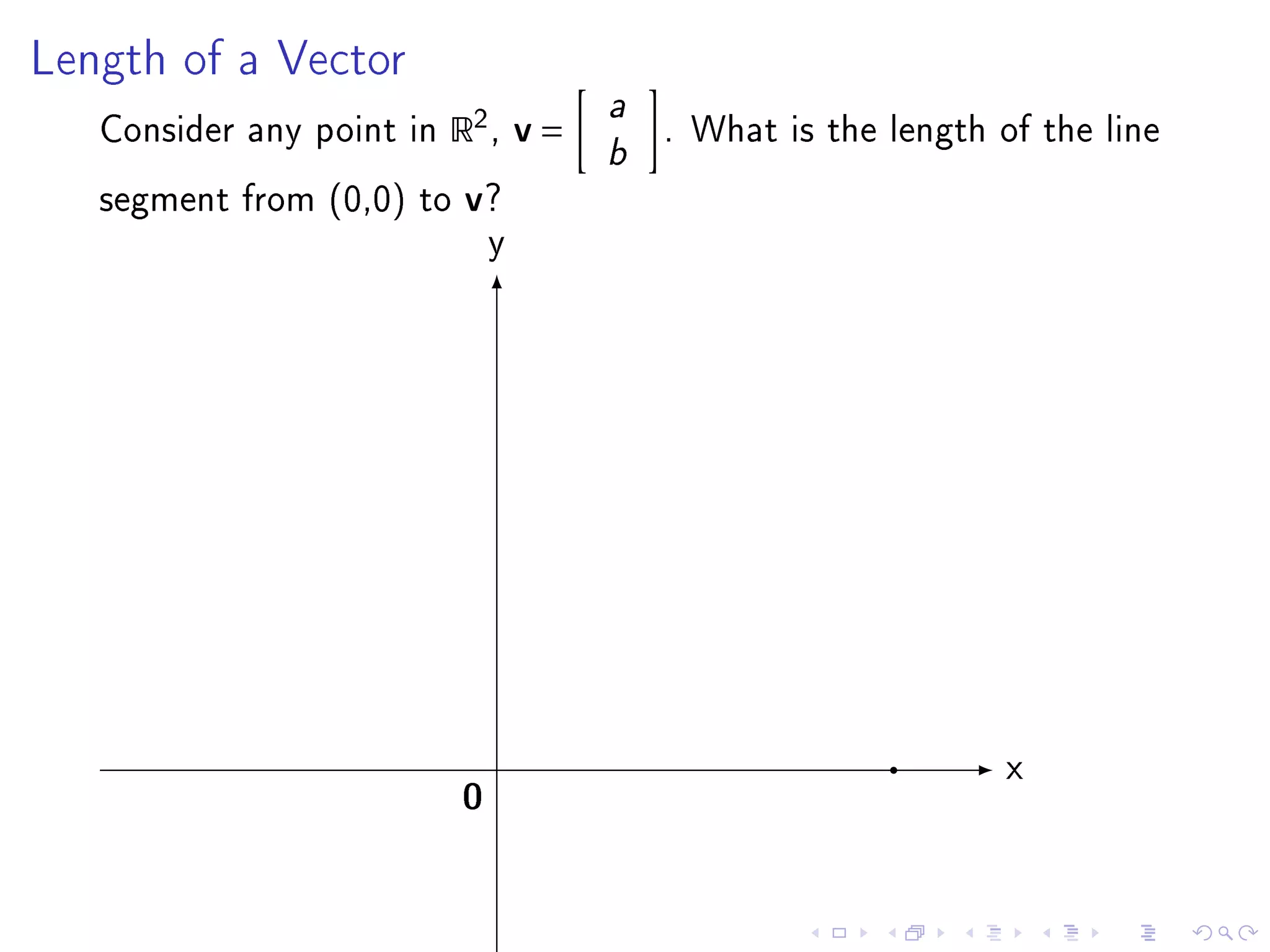
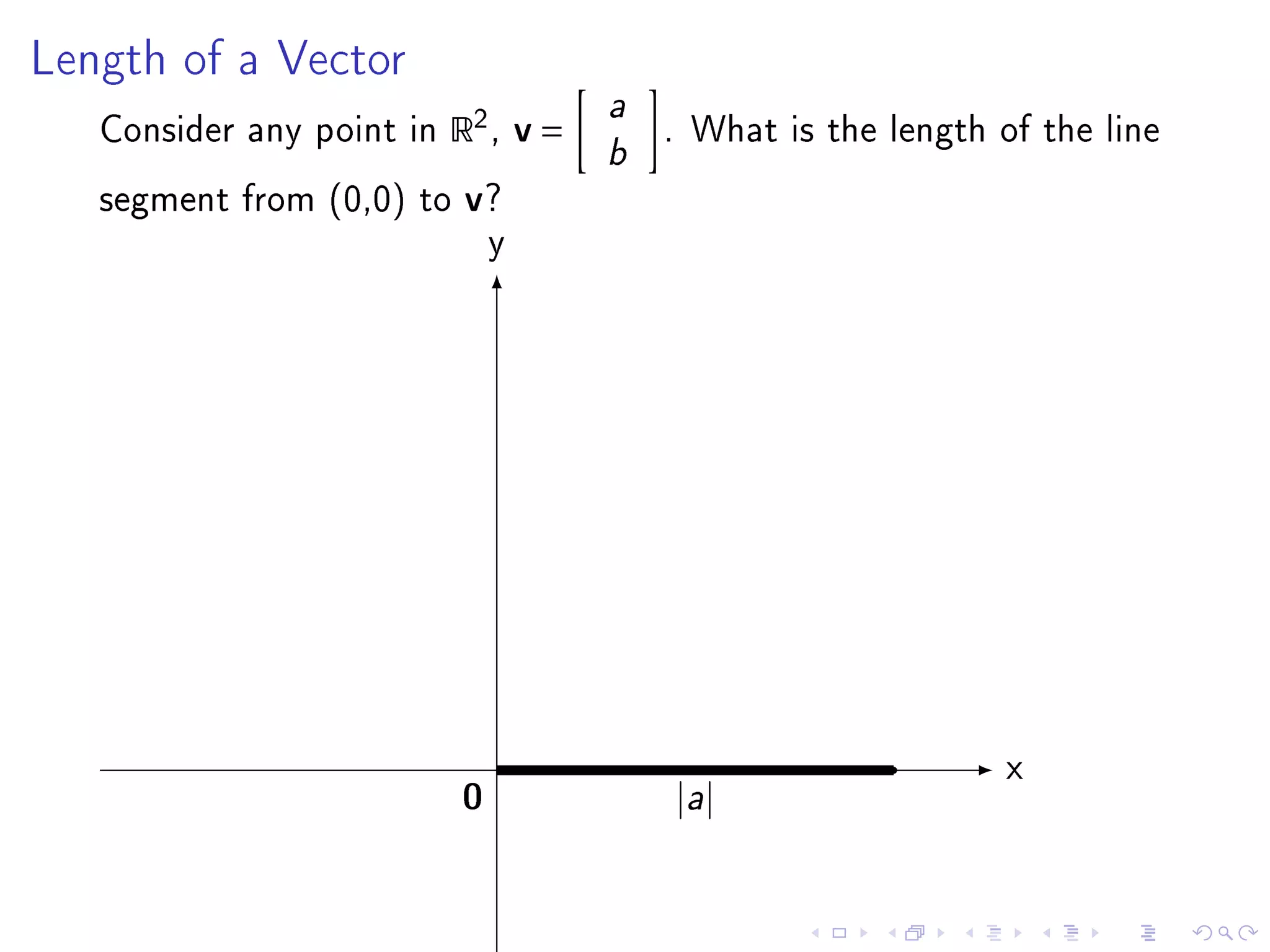
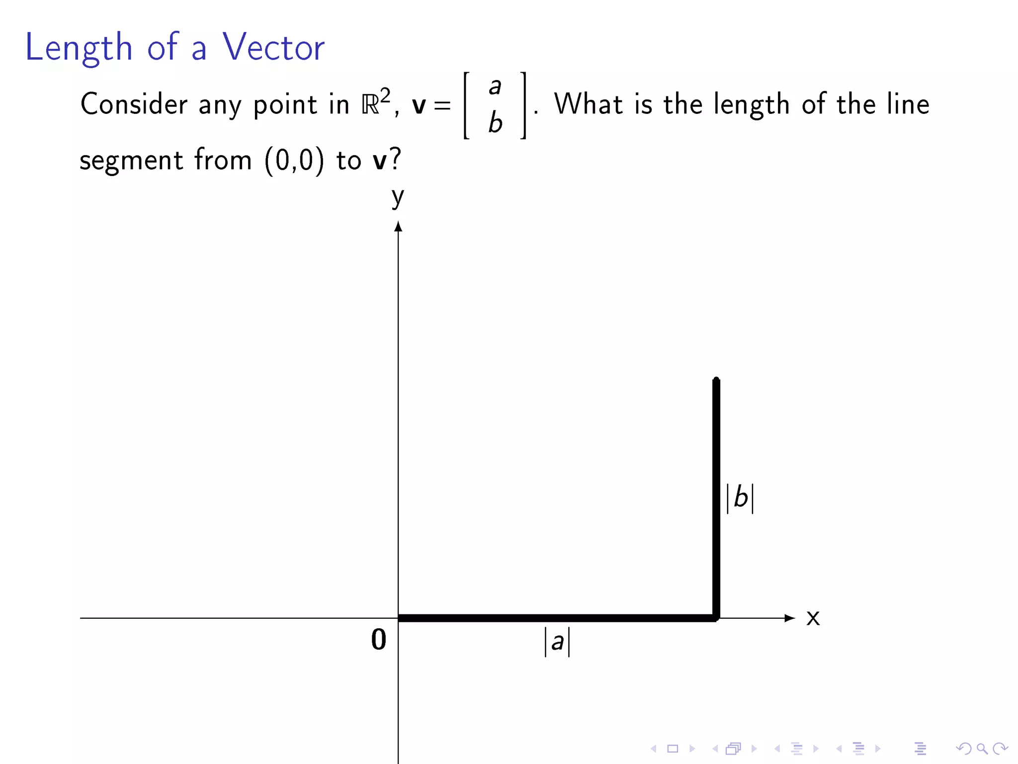
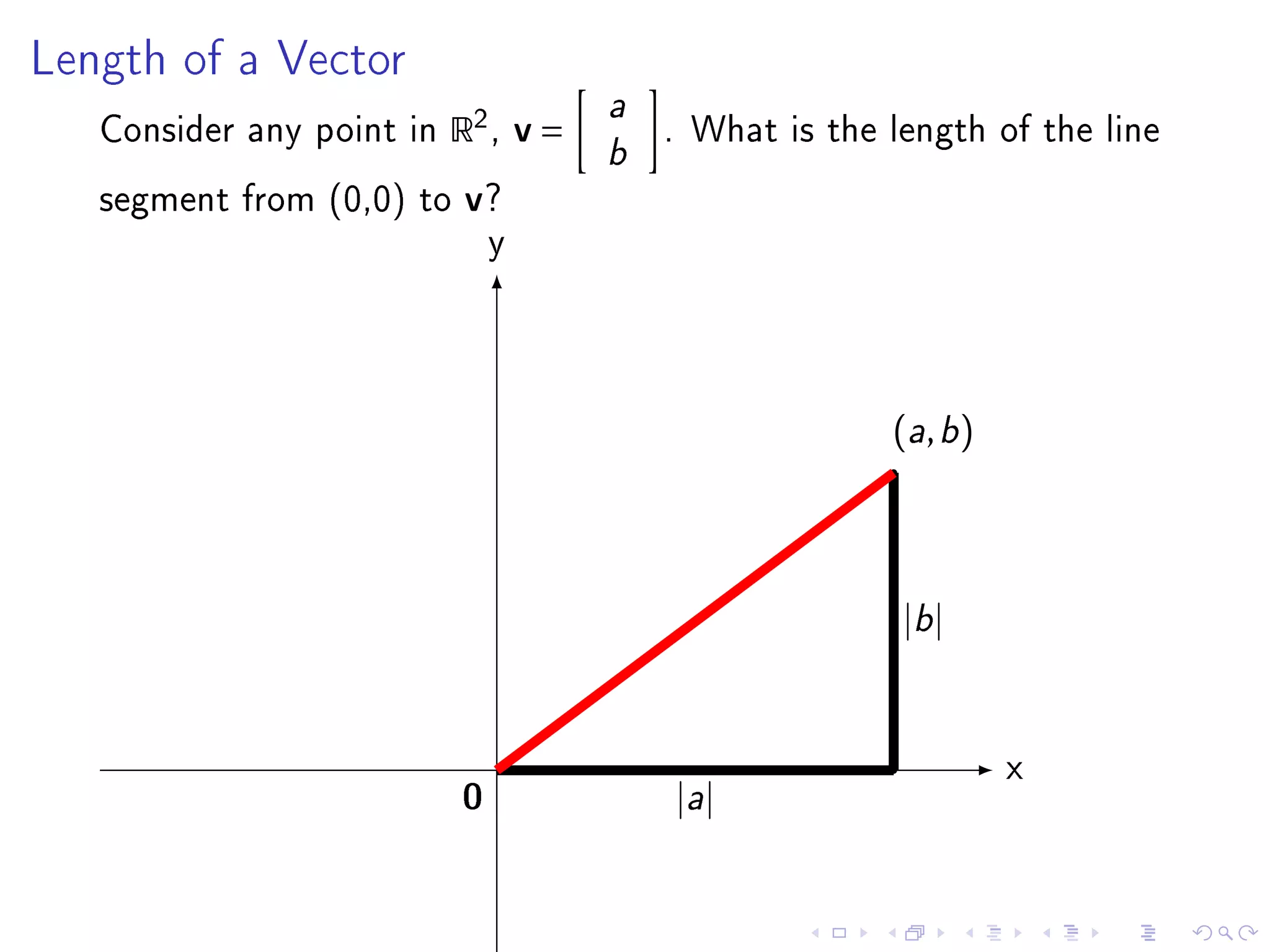
- Quiz 4 will be tomorrow covering sections 3.3, 5.1, and 5.2 of the textbook. It will include 3 problems on Cramer's rule, finding eigenvectors given eigenvalues, and finding characteristic polynomials/eigenvalues of 2x2 and 3x3 matrices. Students must show all work. - Chapter 6 objectives include extending geometric concepts like length, distance, and perpendicularity to Rn. These concepts are useful for least squares fitting of experimental data to a system of equations. 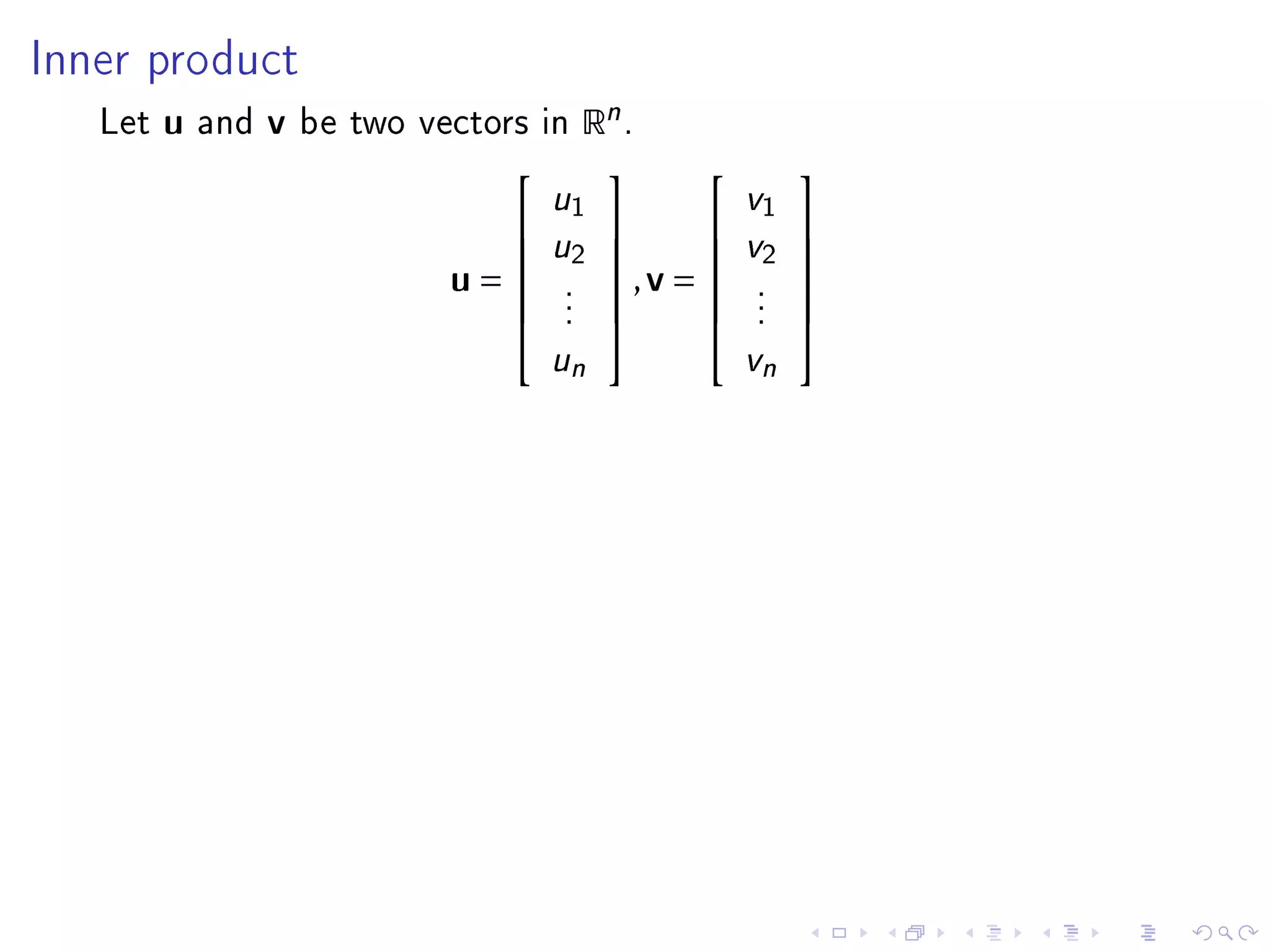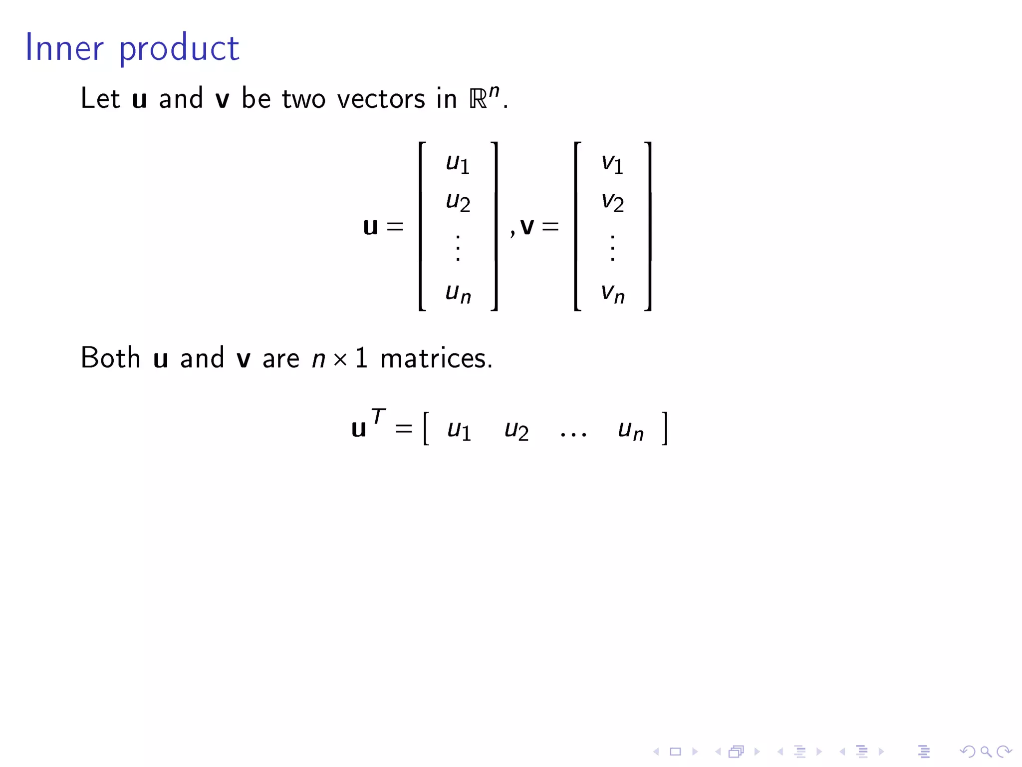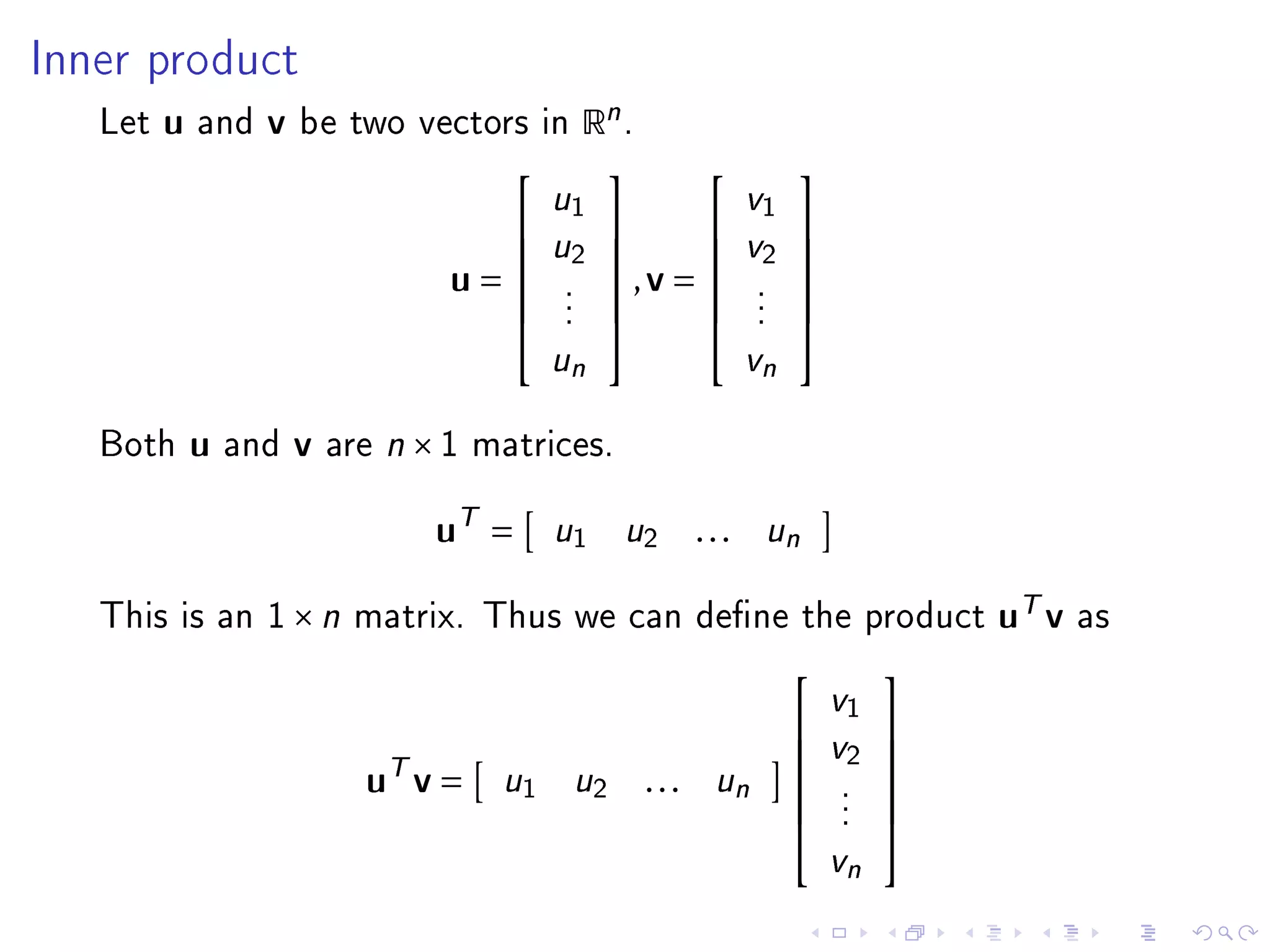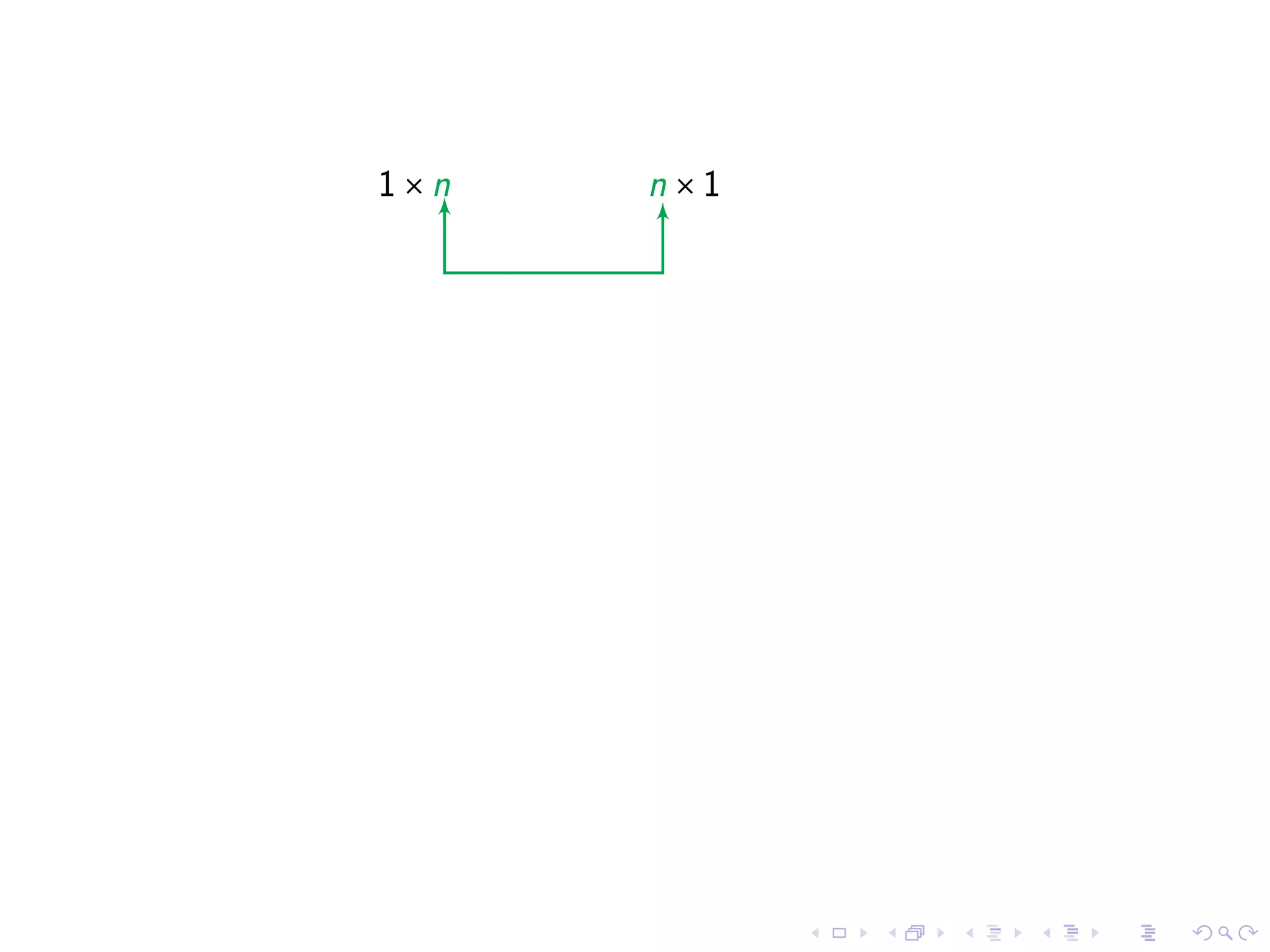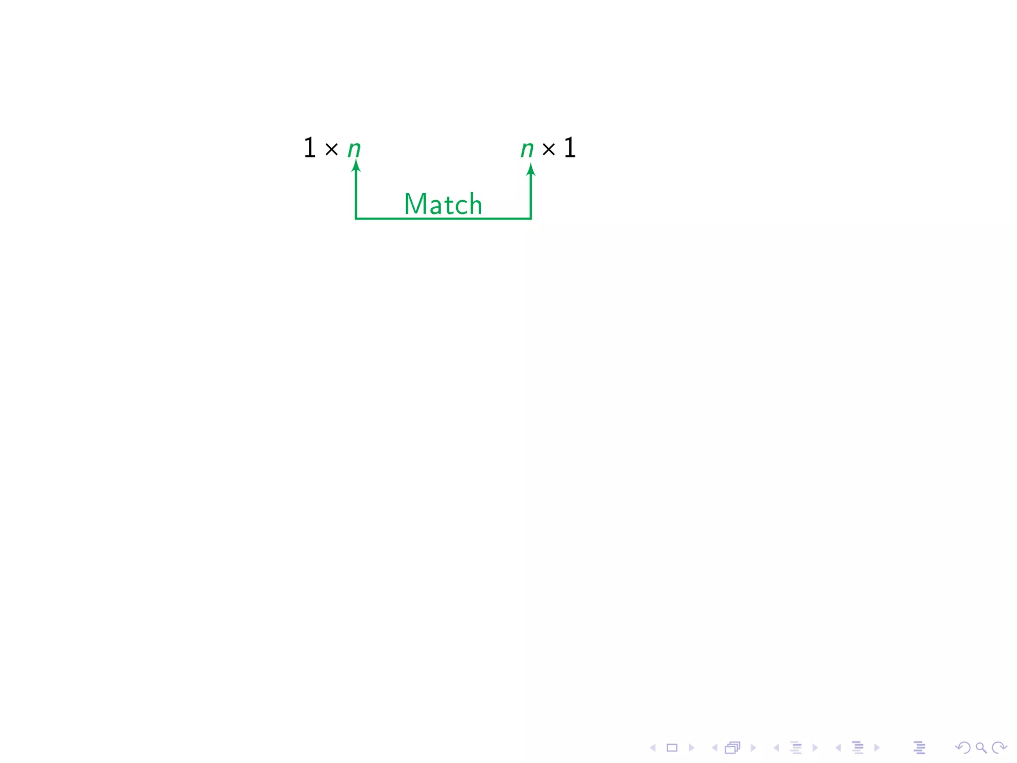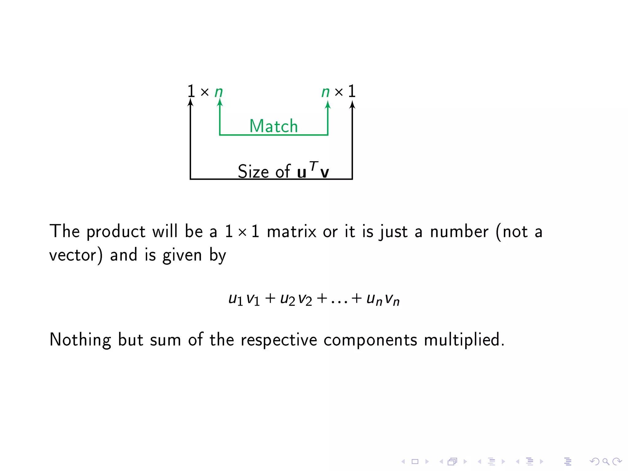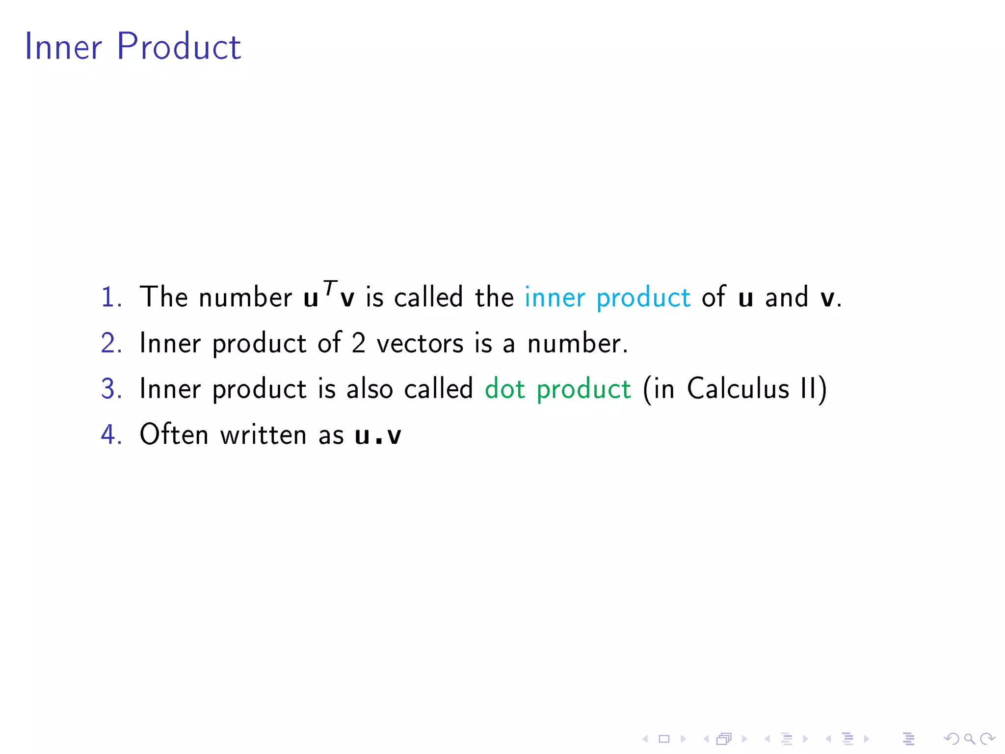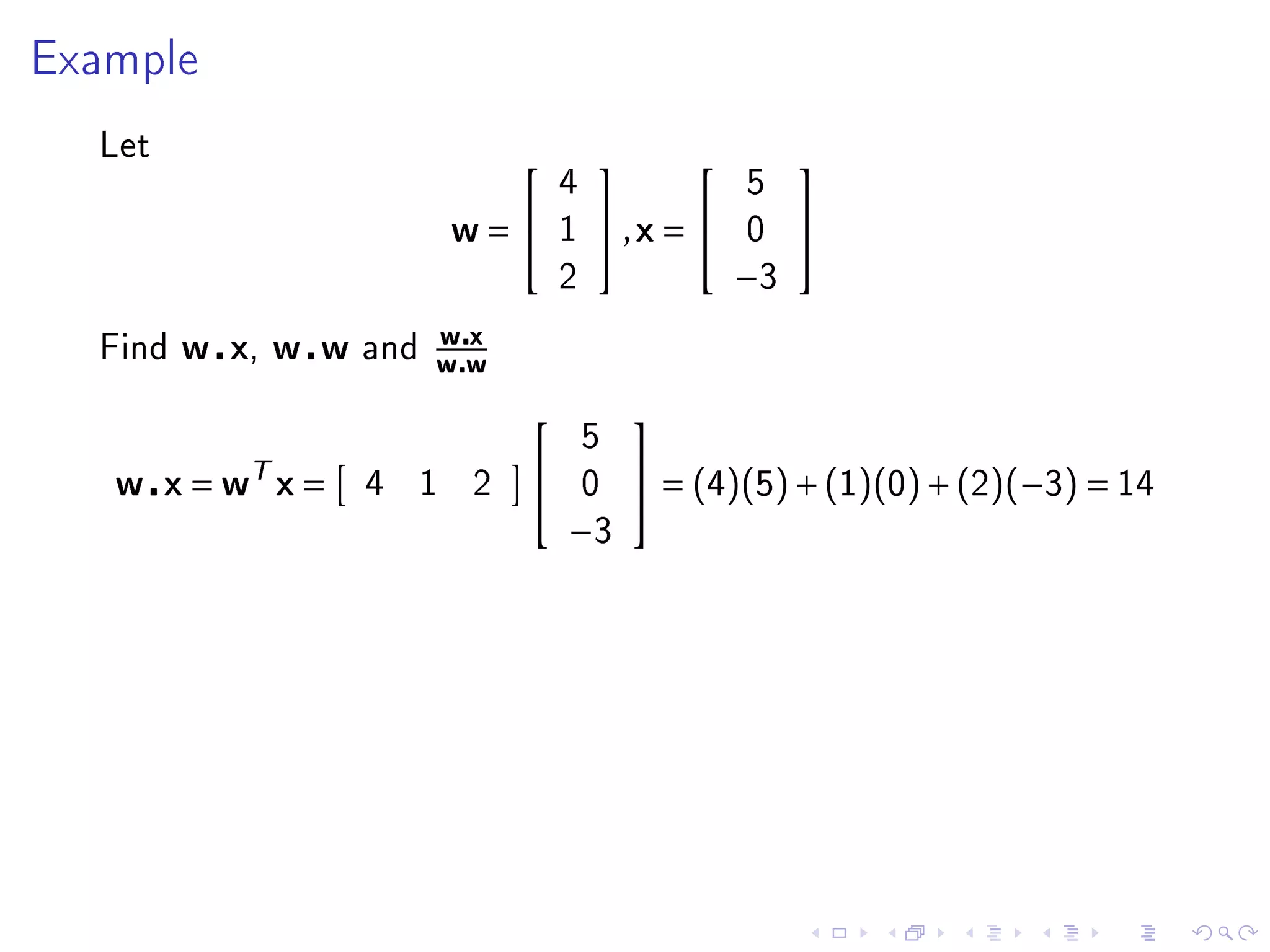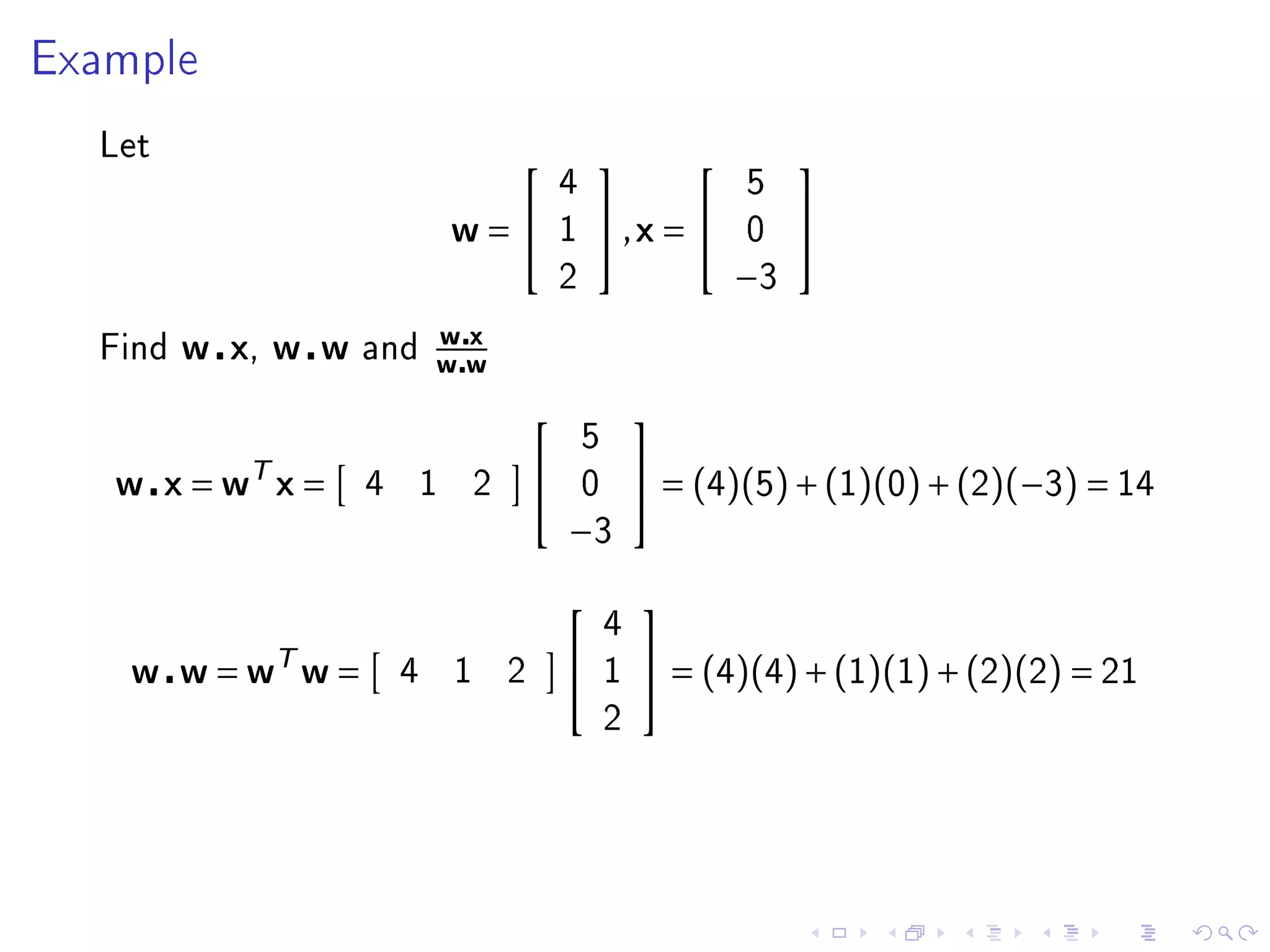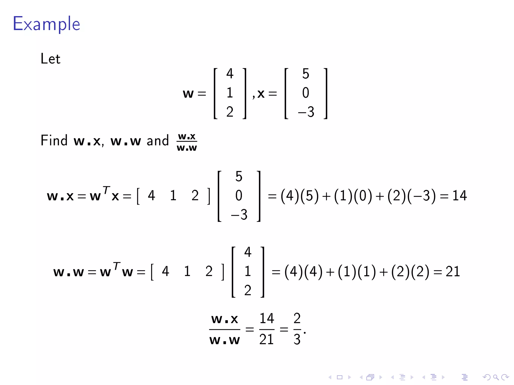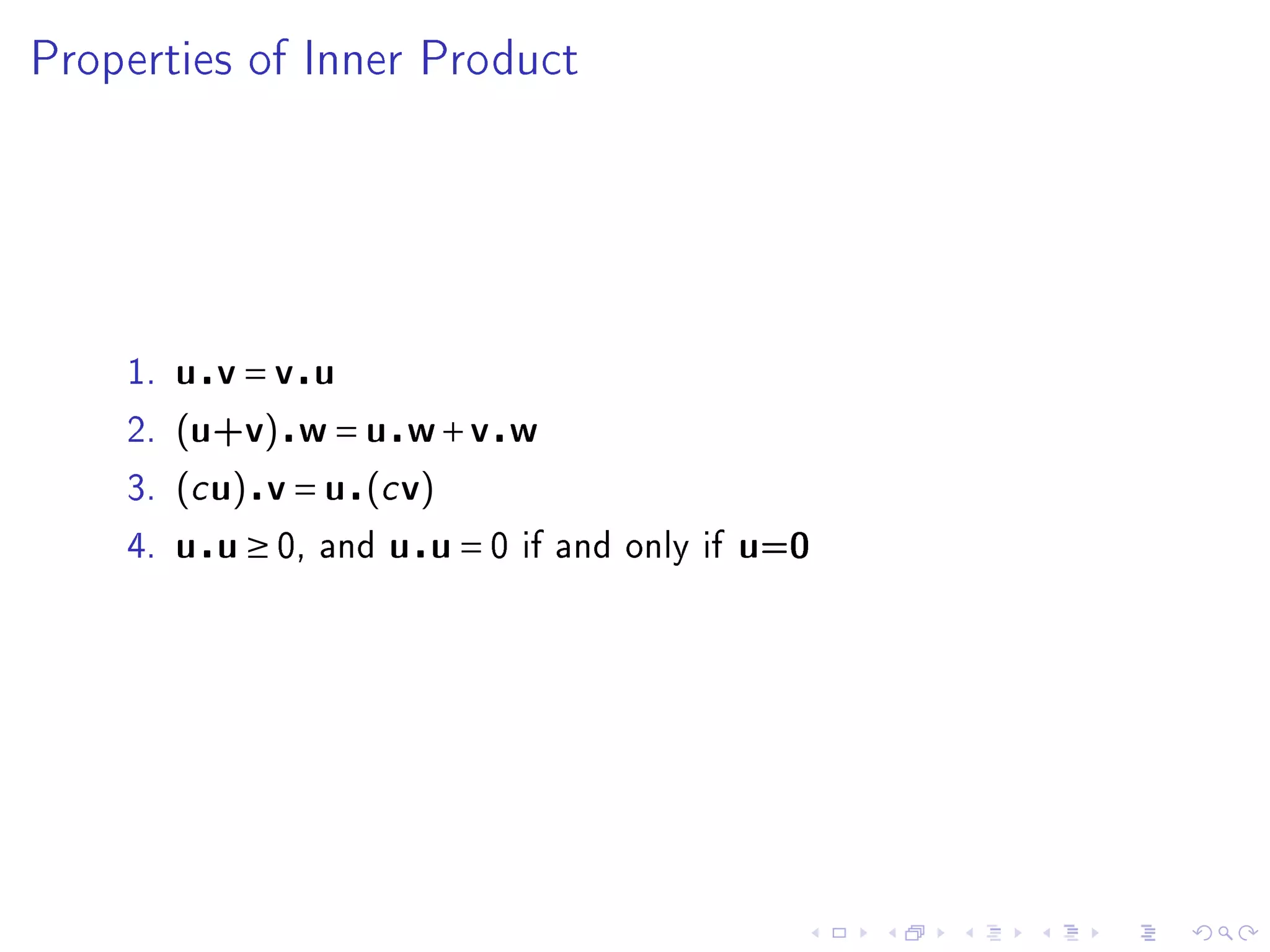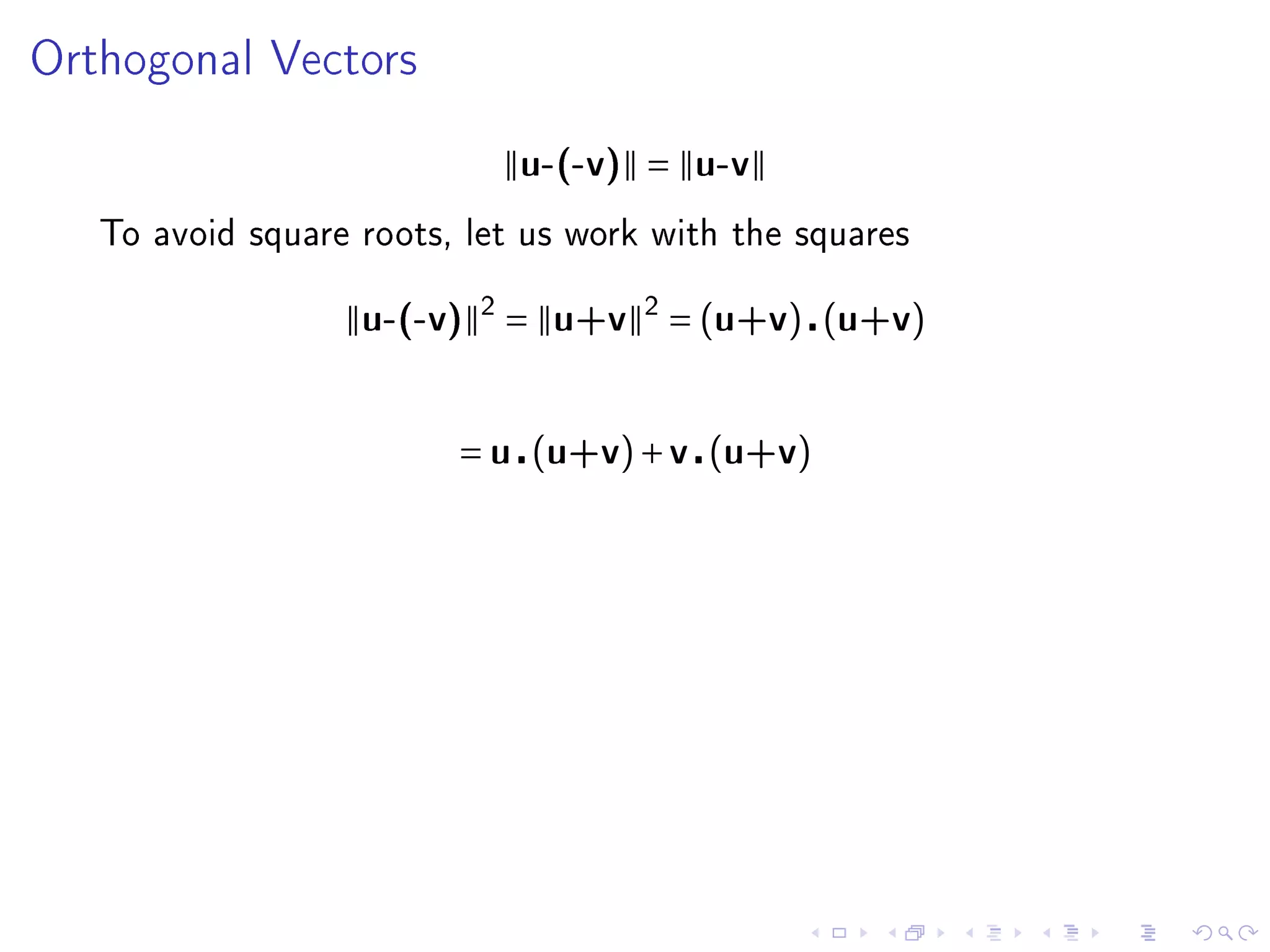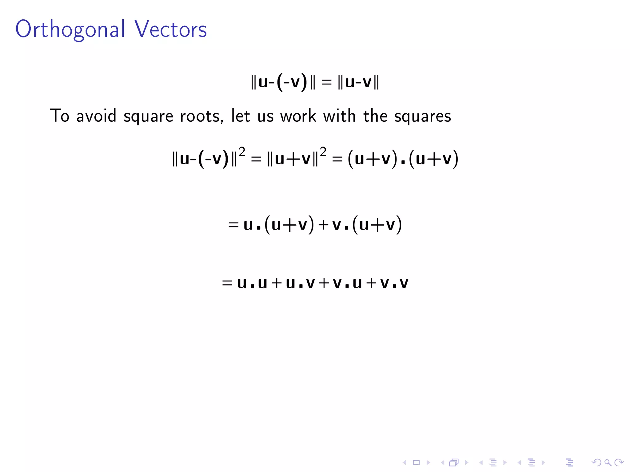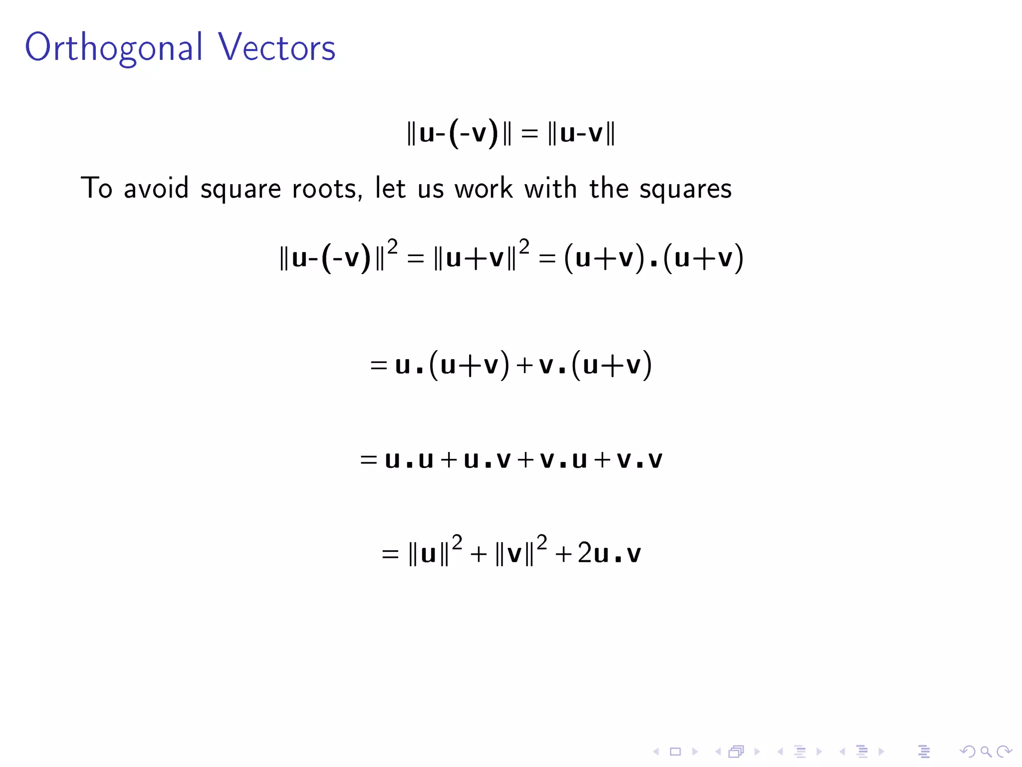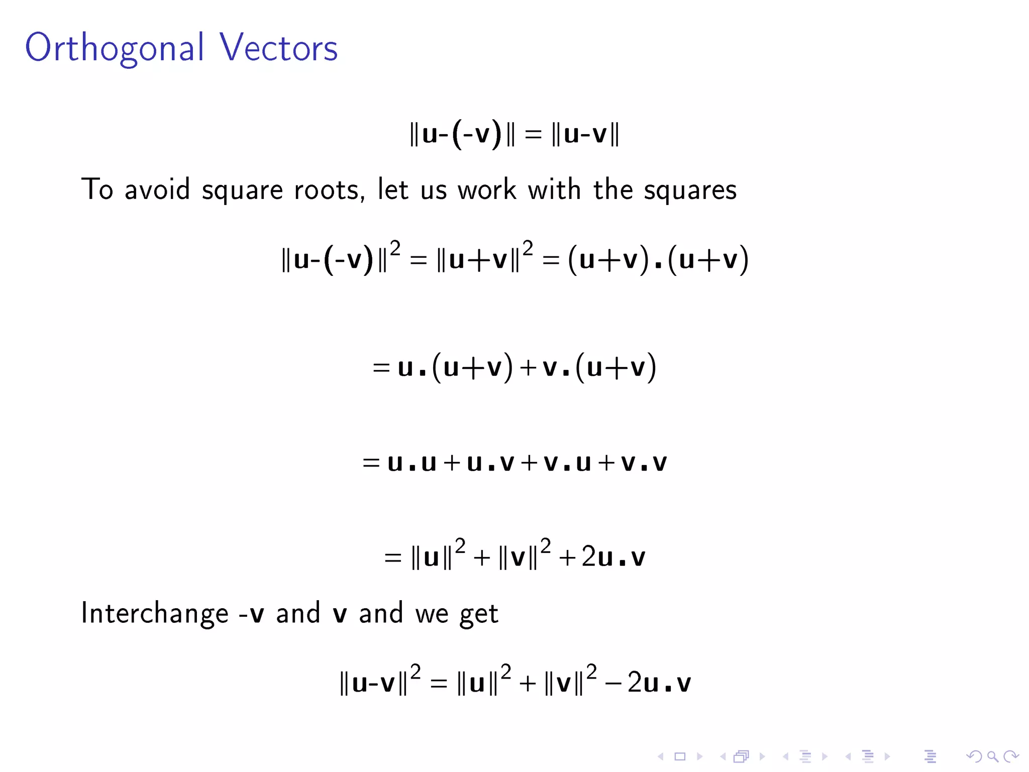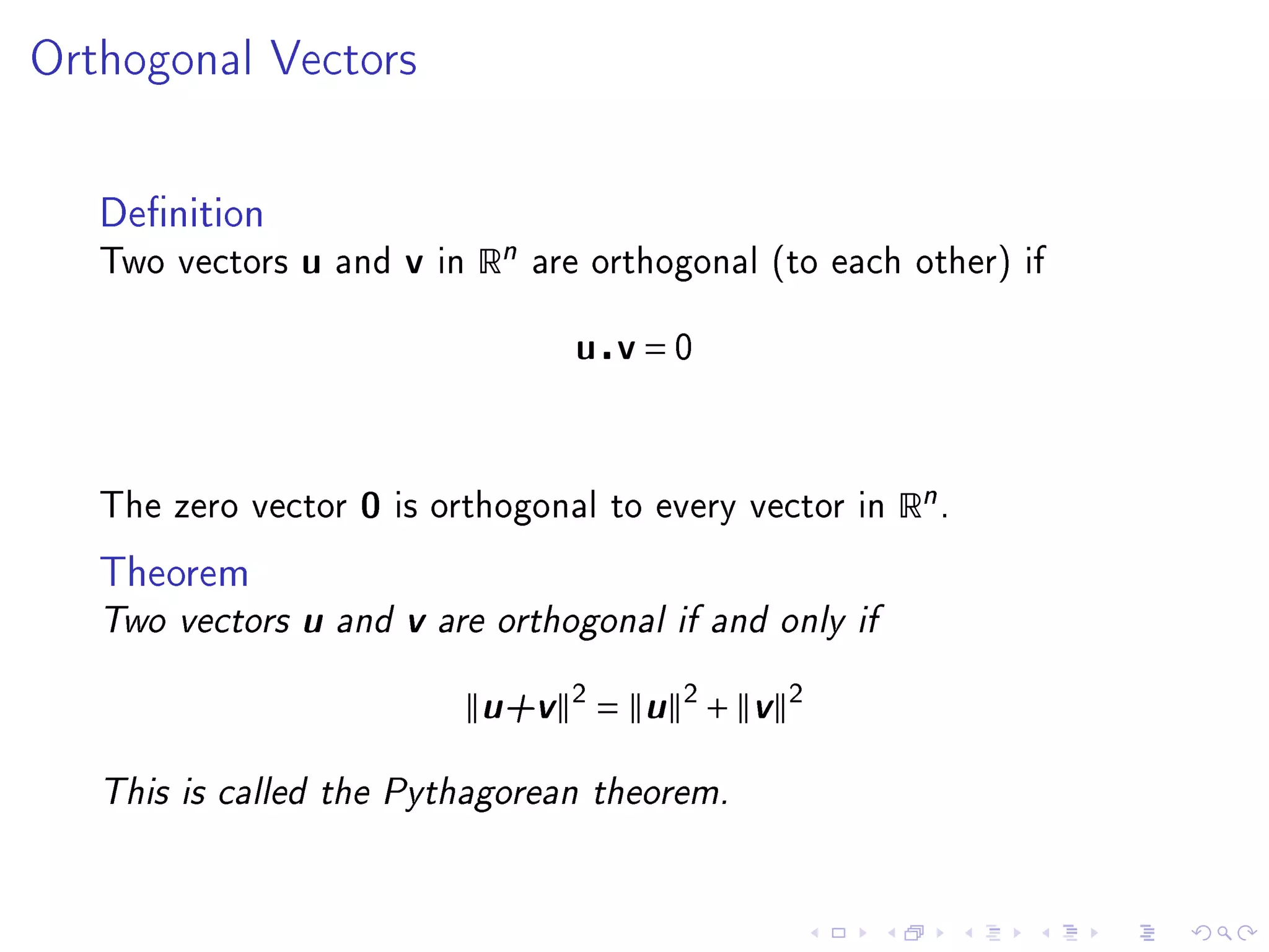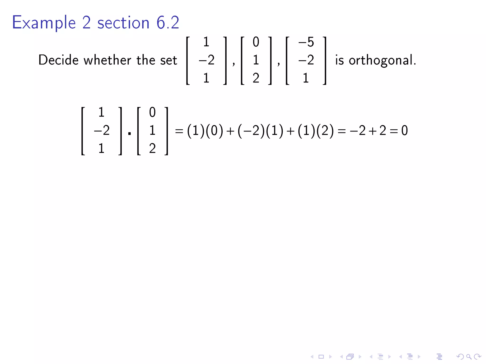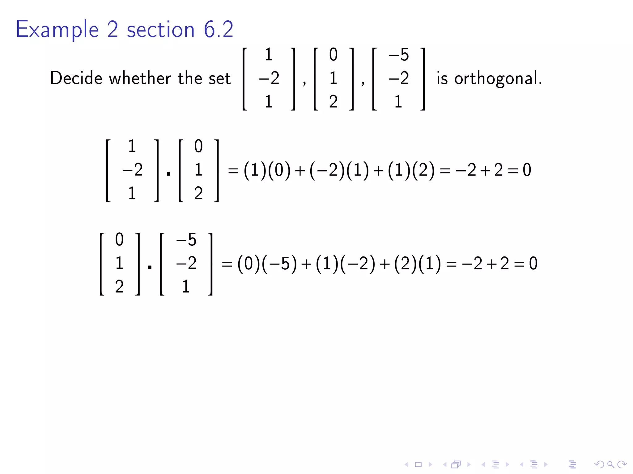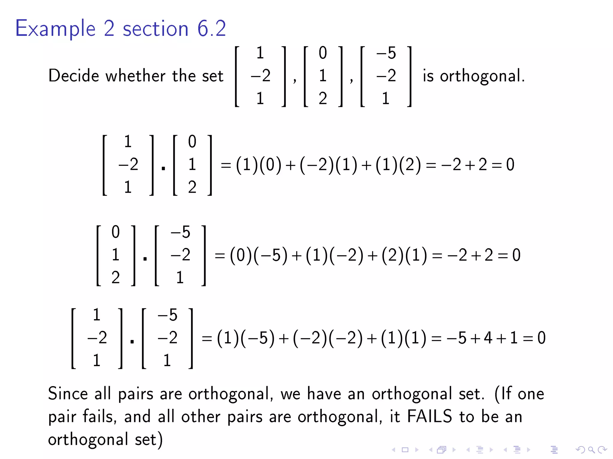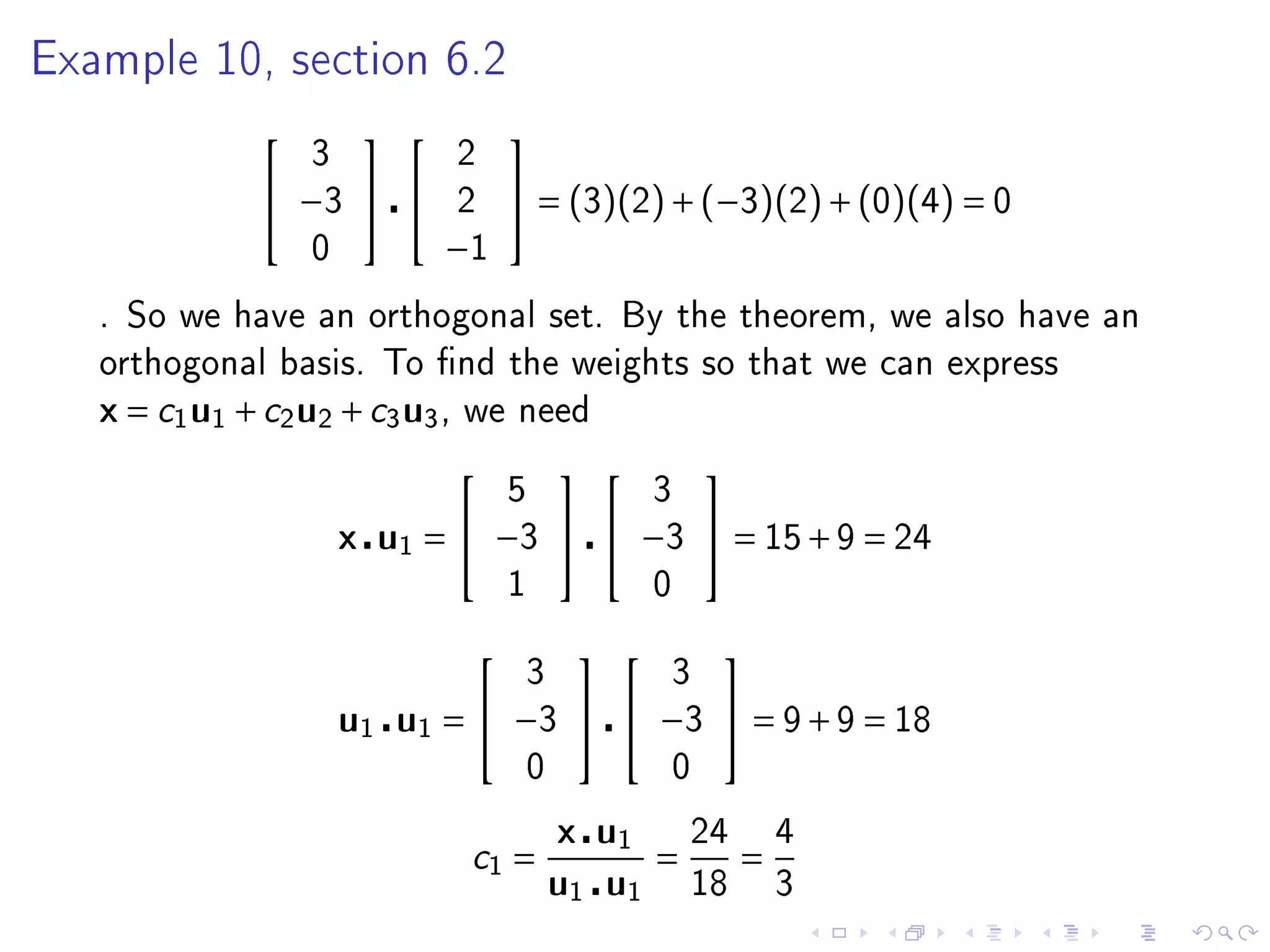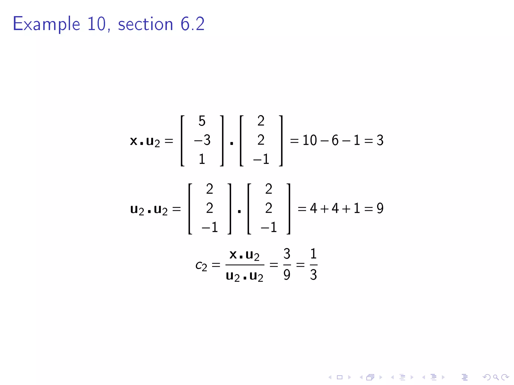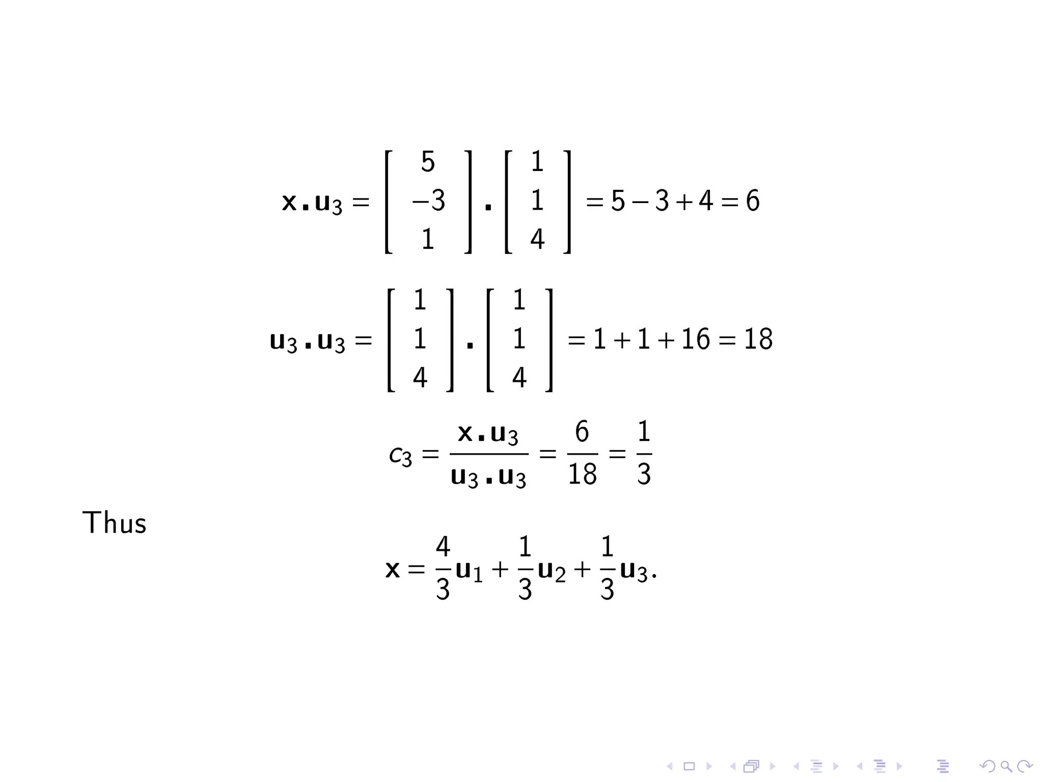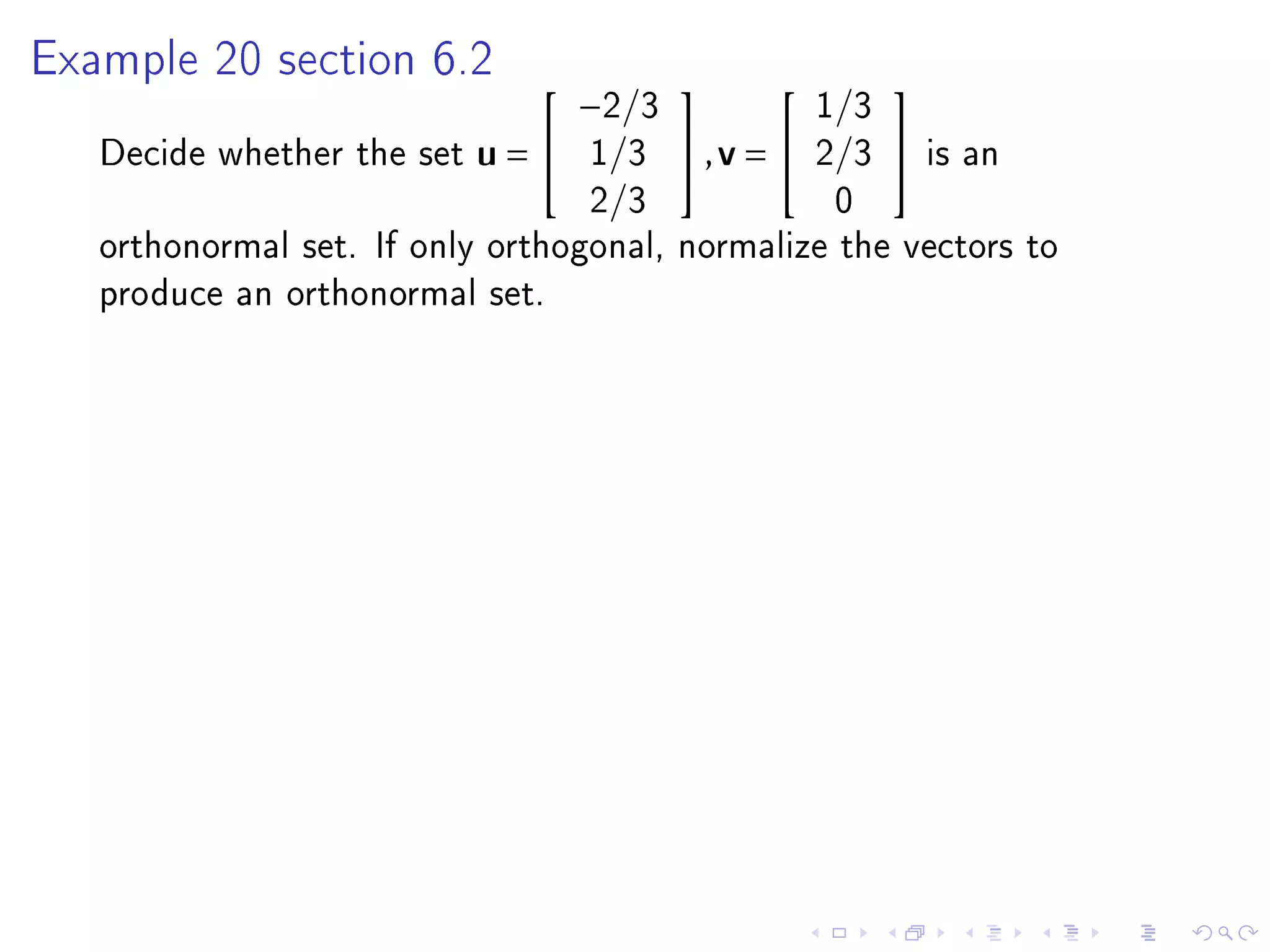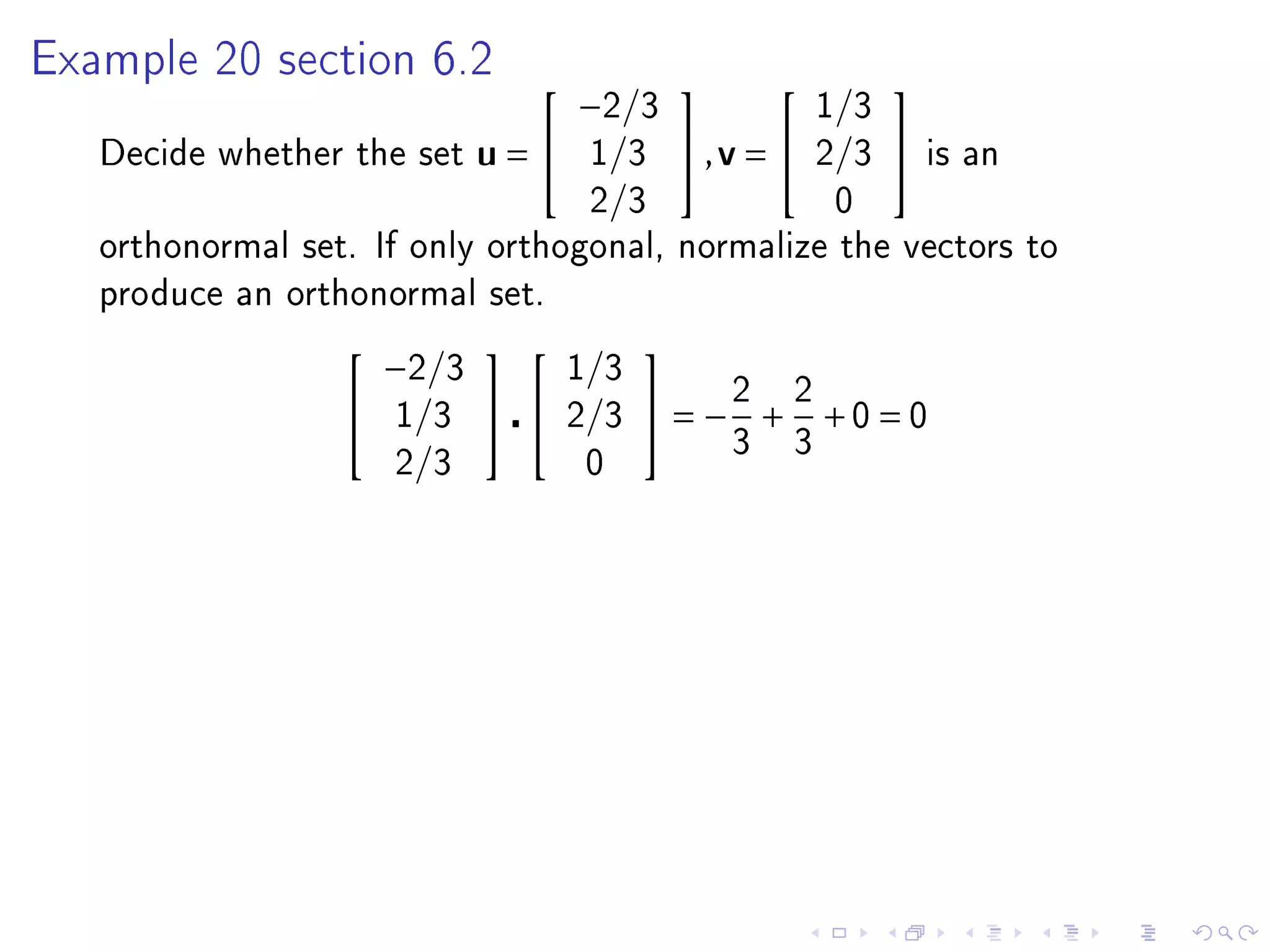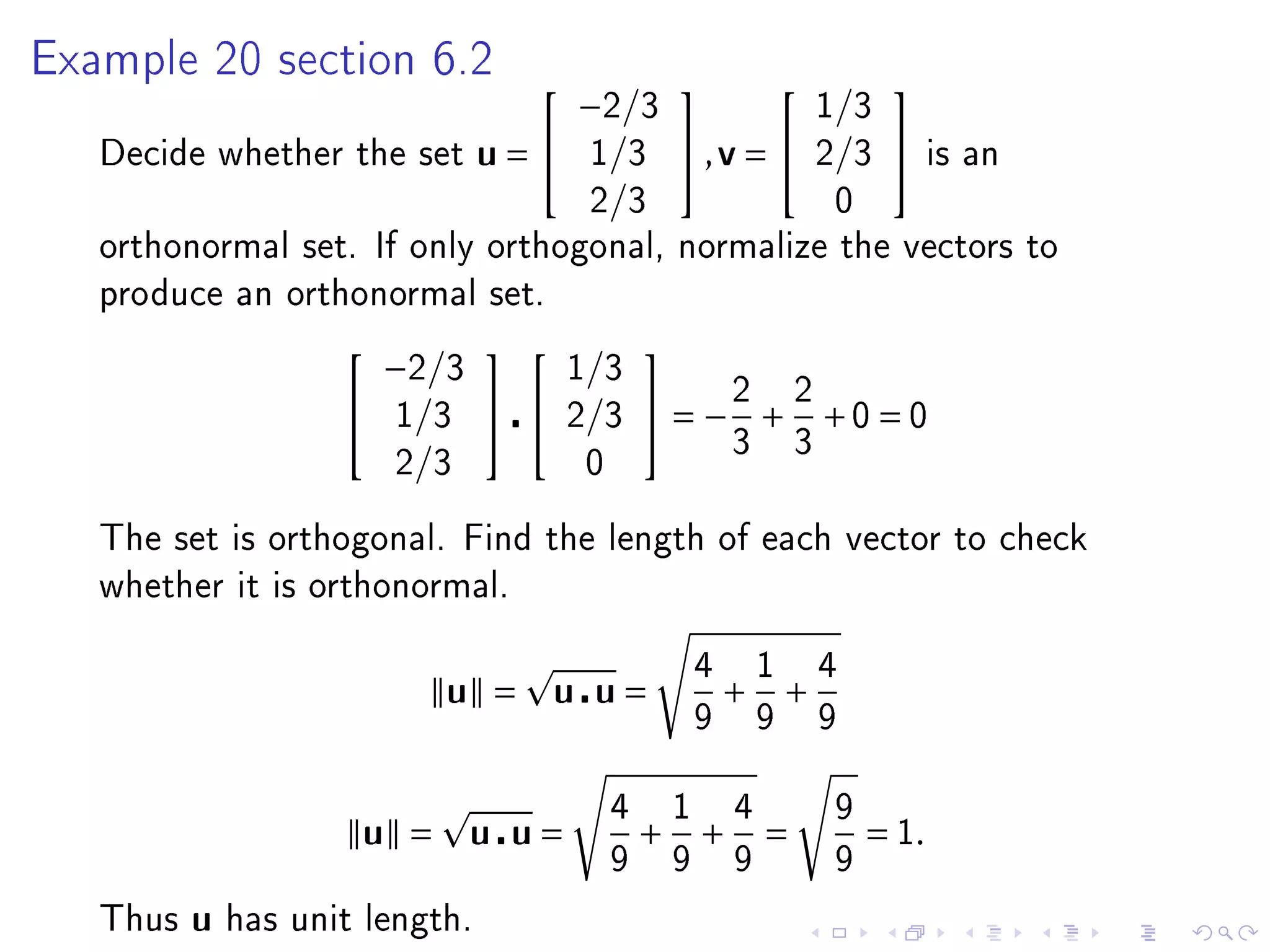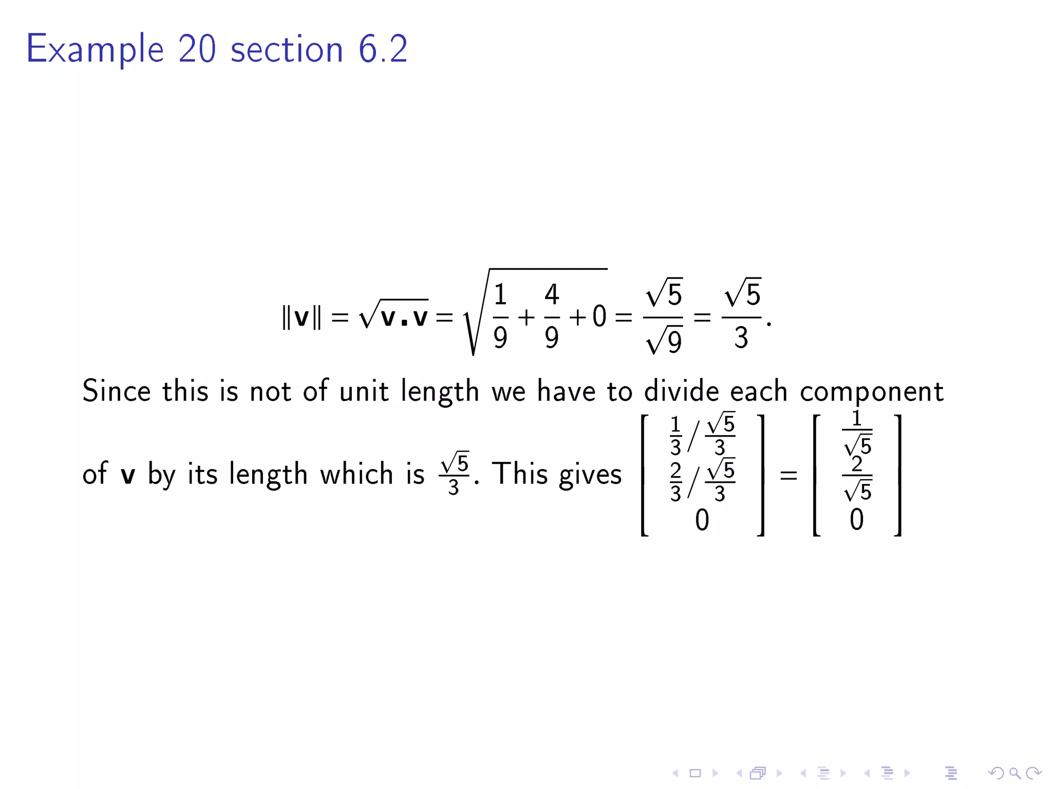- The inner product of two vectors u and v in Rn is defined as their dot product, which is the sum of the component-wise products of corresponding elements in u and v.

1. Announcements
Quiz 4 (last quiz of the term) tomorrow on sec 3.3, 5.1 and
5.2.
Three problems on tomorrow's quiz(Cramer's rule/adjugate,
nding eigenvector(s) given one or more eigenvalue(s), nding
char polynomial/eigenvalues of a 2 × 2 or a nice 3 × 3 matrix.)
You must show all relevant work on the quiz. Calculator
answers are not acceptable.

2. Chapter 6 Orthogonality
Objectives
1. Extend the idea of simple geometric ideas namely length,
distance and perpendicularity from R2 and R3 into Rn

3. Chapter 6 Orthogonality
Objectives
1. Extend the idea of simple geometric ideas namely length,
distance and perpendicularity from R2 and R3 into Rn
2. Useful in tting experimental data of a system Ax = b. If x1
is an acceptable solution, we want the distance between b and
Ax1 to be minimum (or minimize the error)

4. Chapter 6 Orthogonality
Objectives
1. Extend the idea of simple geometric ideas namely length,
distance and perpendicularity from R2 and R3 into Rn
2. Useful in tting experimental data of a system Ax = b. If x1
is an acceptable solution, we want the distance between b and
Ax1 to be minimum (or minimize the error)
3. The solution above is called the least-squares solution and is
widely used where experimental data is scattered over a wide
range and you want to t a straight line.

5. Inner product
Let u and v be two vectors in Rn .
   
u1 v1
 u2   v2 
   
u= .
,v =  .

. .
. .
   
   
un vn

6. Inner product
Let u and v be two vectors in Rn .
   
u1 v1
 u2   v2 
   
u= .
,v =  .

. .
. .
   
   
un vn
Both u and v are n × 1 matrices.
uT = u1 u2 . . . un

7. Inner product
Let u and v be two vectors in Rn .
   
u1 v1
 u2   v2 
   
u= .
,v =  .

. .
. .
   
   
un vn
Both u and v are n × 1 matrices.
uT = u1 u2 . . . un
This is an 1 × n matrix. Thus we can dene the product uT v as
 
v1
 v2 
uT v =
 
u1 u2 . . . un  .

.
.
 
 
vn

8. 1×n n×1

9. 1×n n×1
Match

10. 1×n n×1
Match
Size of uT v
The product will be a 1 × 1 matrix or it is just a number (not a
vector) and is given by
u1 v1 + u2 v2 + . . . + un vn
Nothing but sum of the respective components multiplied.

11. Inner Product
1. The number uT v is called the inner product of u and v.
2. Inner product of 2 vectors is a number.
3. Inner product is also called dot product (in Calculus II)
4. Often written as u v

12. Example
Let
   
4 5
w= 1 ,x =  0 
2 −3
wx
Find w x, w w and
ww

13. Example
Let
   
4 5
w= 1 ,x =  0 
2 −3
wx
Find w x, w w and
ww
 
5
w x = wT x = 4 1 2  0  = (4)(5) + (1)(0) + (2)(−3) = 14
−3

14. Example
Let
   
4 5
w= 1 ,x =  0 
2 −3
wx
Find w x, w w and
ww
 
5
w x = wT x = 4 1 2  0  = (4)(5) + (1)(0) + (2)(−3) = 14
−3
 
4
w w = wT w = 4 1 2  1  = (4)(4) + (1)(1) + (2)(2) = 21
2

15. Example
Let
   
4 5
w= 1 ,x =  0 
2 −3
wx
Find w x, w w and
ww
 
5
w x = wT x = 4 1 2  0  = (4)(5) + (1)(0) + (2)(−3) = 14
−3
 
4
w w = wT w = 4 1 2  1  = (4)(4) + (1)(1) + (2)(2) = 21
2
w x 14 2
= = .
w w 21 3

16. Properties of Inner Product
1. u v=v u
2. (u+v) w = u w + v w
3. (c u) v = u (c v)
4. u u ≥ 0, and u u=0 if and only if u=0

17. Length of a Vector
a
Consider any point in R2 , v = . What is the length of the line
b
segment from (0,0) to v?
y
x
0

18. Length of a Vector
a
Consider any point in R2 , v = . What is the length of the line
b
segment from (0,0) to v?
y
x
0 |a |

19. Length of a Vector
a
Consider any point in R2 , v = . What is the length of the line
b
segment from (0,0) to v?
y
|b |
x
0 |a |

20. Length of a Vector
a
Consider any point in R2 , v = . What is the length of the line
b
segment from (0,0) to v?
y
(a, b)
|b |
x
0 |a |

21. Length of a Vector
a
Consider any point in R2 , v = . What is the length of the line
b
segment from (0,0) to v?
y
(a, b)
a2 + b 2
|b |
x
0 |a |

22. Length of a Vector
 
v1
 v2 
 
We can extend this idea to Rn , where v= .
.
.
.
 
 
vn
Denition
The length (or the norm) of v is the nonnegative scalar v dened
by
v = v v= 2 2 2
v1 + v2 + . . . + vn
Since we have sum of squares of the components, the square root is
always dened.

23. Length of a Vector
If c is a scalar, the length of c v is c times the length of v. If c 1,
the vector is stretched by c units and if c 1, c shrinks by c units.

24. Length of a Vector
If c is a scalar, the length of c v is c times the length of v. If c 1,
the vector is stretched by c units and if c 1, c shrinks by c units.
Denition
A vector of length 1 is called a unit vector.

25. Length of a Vector
If c is a scalar, the length of c v is c times the length of v. If c 1,
the vector is stretched by c units and if c 1, c shrinks by c units.
Denition
A vector of length 1 is called a unit vector.
1
If we divide a vector v by its length v (or multiply by
v ), we get
the unit vector u in the direction of v.

26. Length of a Vector
If c is a scalar, the length of c v is c times the length of v. If c 1,
the vector is stretched by c units and if c 1, c shrinks by c units.
Denition
A vector of length 1 is called a unit vector.
1
If we divide a vector v by its length v (or multiply by
v ), we get
the unit vector u in the direction of v.
The process of getting u from v is called normalizing v.

27. Example 10, sec 6.1
 
−6
Find a unit vector in the direction of v= 4 .
−3
To compute the length of v, rst nd
v v = (−6)2 + 42 + (−3)2 = 36 + 16 + 9 = 61

28. Example 10, sec 6.1
 
−6
Find a unit vector in the direction of v= 4 .
−3
To compute the length of v, rst nd
v v = (−6)2 + 42 + (−3)2 = 36 + 16 + 9 = 61
Then,
v = 61

29. Example 10, sec 6.1
 
−6
Find a unit vector in the direction of v= 4 .
−3
To compute the length of v, rst nd
v v = (−6)2 + 42 + (−3)2 = 36 + 16 + 9 = 61
Then,
v = 61
The unit vector in the direction of v is
 
−6/
 
−6 61
1 1
u= v= 4 = 4/ 61
 
v
 
61
−3 −3/ 61

30. Distance in Rn
In R (the set of real numbers), the distance between 2 numbers is
easy.
The distance between 4 and 15 is |4 − 14| = | − 10| = 10 or
|14 − 4| = |10| = 10.

31. Distance in Rn
In R (the set of real numbers), the distance between 2 numbers is
easy.
The distance between 4 and 15 is |4 − 14| = | − 10| = 10 or
|14 − 4| = |10| = 10.
Similarly the distance between -5 and 5 is | − 5 − 5| = | − 10| = 10 or
|5 − (−5)| = |10| = 10
Distance has a direct analogue in Rn .

32. Distance in Rn
Denition
For any two vectors u and v in Rn , the distance between u and v
written as dist(u,v) is the length of the vector u-v.
dist(u, v) = u-v

33. Example 14, sec 6.1
   
0 −4
Find the distance between u =  −5  and v =  −1 .
2 8
To compute the distance between u and v, rst nd
     
0 −4 4
u − v =  −5  −  −1  =  −4 
2 8 −6
Then,
u-v = 16 + 16 + 36 = 68

34. Orthogonal Vectors
v
0
-v

35. Orthogonal Vectors
u
v
0
-v
If the 2 green lines are perpendicular, u must have the same
distance from v and -v

36. Orthogonal Vectors
u
u-v
v
u-(-v)
0
-v
If the 2 green lines are perpendicular, u must have the same
distance from v and -v

37. Orthogonal Vectors
u-(-v) = u-v
To avoid square roots, let us work with the squares
u-(-v) 2 = u+v 2 = (u+v) (u+v)

38. Orthogonal Vectors
u-(-v) = u-v
To avoid square roots, let us work with the squares
u-(-v) 2 = u+v 2 = (u+v) (u+v)
= u (u+v) + v (u+v)

39. Orthogonal Vectors
u-(-v) = u-v
To avoid square roots, let us work with the squares
u-(-v) 2 = u+v 2 = (u+v) (u+v)
= u (u+v) + v (u+v)
= u u+u v+v u+v v

40. Orthogonal Vectors
u-(-v) = u-v
To avoid square roots, let us work with the squares
u-(-v) 2 = u+v 2 = (u+v) (u+v)
= u (u+v) + v (u+v)
= u u+u v+v u+v v
= u 2 + v 2 + 2u v

41. Orthogonal Vectors
u-(-v) = u-v
To avoid square roots, let us work with the squares
u-(-v) 2 = u+v 2 = (u+v) (u+v)
= u (u+v) + v (u+v)
= u u+u v+v u+v v
= u 2 + v 2 + 2u v
Interchange -v and v and we get
u-v 2 = u 2 + v 2 − 2u v

42. Orthogonal Vectors
Equate the 2 expressions,
u 2 + v 2 + 2u v = u 2 + v 2 − 2u v
=⇒ 2u v = −2u v
=⇒ u v = 0

43. Orthogonal Vectors
Equate the 2 expressions,
u 2 + v 2 + 2u v = u 2 + v 2 − 2u v
=⇒ 2u v = −2u v
=⇒ u v = 0
If u and v are points in R2 , the lines through these points and (0,0)
are perpendicular if and only if
u v=0

44. Orthogonal Vectors
Equate the 2 expressions,
u 2 + v 2 + 2u v = u 2 + v 2 − 2u v
=⇒ 2u v = −2u v
=⇒ u v = 0
If u and v are points in R2 , the lines through these points and (0,0)
are perpendicular if and only if
u v=0
Generalize this idea of perpendicularity to Rn . We use the word
orthogonality in linear algebra for perpendicularity.

45. Orthogonal Vectors
Denition
Two vectors u and v in Rn are orthogonal (to each other) if
u v=0
The zero vector 0 is orthogonal to every vector in Rn .

46. Orthogonal Vectors
Denition
Two vectors u and v in Rn are orthogonal (to each other) if
u v=0
The zero vector 0 is orthogonal to every vector in Rn .
Theorem
Two vectors u and v are orthogonal if and only if
u+v 2 = u 2 + v 2
This is called the Pythagorean theorem.

47. Example 16, 18 section 6.1
Decide which pair(s) of vectors are orthogonal
   
12 2
16)u =  3  , v =  −3 
−5 3
u v = (12)(2) + (3)(−3) + (−5)(3) = 24 − 9 − 15 = 0.
Thus u and v are orthogonal.

48. Example 16, 18 section 6.1
Decide which pair(s) of vectors are orthogonal
   
12 2
16)u =  3  , v =  −3 
−5 3
u v = (12)(2) + (3)(−3) + (−5)(3) = 24 − 9 − 15 = 0.
Thus uand vare orthogonal.
 
−3 1
 7
  −8 
18)y =  ,z = 
   
4  15

  
0 −7
y z = (−3)(1) + (7)(−8) + (4)(15) + (0)(−7) = −3 − 56 + 60 − 0 = 1 = 0.
Thus y and z are not orthogonal.

49. Orthogonal Complement
Let W be a subspace of Rn . If any vector z is orthogonal to every
vector in W , we say that z is orthogonal to W .
There could be more than one such vector z which is orthogonal to
W.

50. Orthogonal Complement
Let W be a subspace of Rn . If any vector z is orthogonal to every
vector in W , we say that z is orthogonal to W .
There could be more than one such vector z which is orthogonal to
W.
Denition
A collection of all vectors that are orthogonal to W is called the
orthogonal complement of W .

51. Orthogonal Complement
Let W be a subspace of Rn . If any vector z is orthogonal to every
vector in W , we say that z is orthogonal to W .
There could be more than one such vector z which is orthogonal to
W.
Denition
A collection of all vectors that are orthogonal to W is called the
orthogonal complement of W .
⊥
The orthogonal complement of W is denoted by W and is read as
W perpendicular or W perp.

52. Orthogonal Complement
⊥
1. A vector x is in W if and only if x is orthogonal to every
vector that spans (generates) W .

53. Orthogonal Complement
⊥
1. A vector x is in W if and only if x is orthogonal to every
vector that spans (generates) W .
2. W
⊥
is a subspace of Rn .

54. Orthogonal Complement
⊥
1. A vector x is in W if and only if x is orthogonal to every
vector that spans (generates) W .
2. W
⊥
is a subspace of Rn .
3. If A is an m × n matrix, the orthogonal complement of Col A is
Nul A
T. (Useful in part (d) of T/F questions, prob 19)

55. Orthogonal Complement
⊥
1. A vector x is in W if and only if x is orthogonal to every
vector that spans (generates) W .
2. W
⊥
is a subspace of Rn .
3. If A is an m × n matrix, the orthogonal complement of Col A is
Nul A
T. (Useful in part (d) of T/F questions, prob 19)
⊥
4. If a vector is in both W and W , then that vector must be
the zero vector. (The only vector perpendicular to itself is the
zero vector)

56. Section 6.2 Orthogonal Sets
Consider a set of vectors u1 , u2 , . . . , up in Rn . If each pair of
distinct vectors from the set is orthogonal (that is u1 u2 = 0,
u1 u3 = 0, u2 u3 = 0 etc etc) then the set is called an orthogonal
set.

57. Example 2 section 6.2
     
1 0 −5
Decide whether the set  −2  ,  1  ,  −2  is orthogonal.
1 2 1

58. Example 2 section 6.2
     
1 0 −5
Decide whether the set  −2  ,  1  ,  −2  is orthogonal.
1 2 1
   
1 0
 −2   1  = (1)(0) + (−2)(1) + (1)(2) = −2 + 2 = 0
1 2

59. Example 2 section 6.2
     
1 0 −5
Decide whether the set  −2  ,  1  ,  −2  is orthogonal.
1 2 1
   
1 0
 −2   1  = (1)(0) + (−2)(1) + (1)(2) = −2 + 2 = 0
1 2
   
0 −5
 1   −2  = (0)(−5) + (1)(−2) + (2)(1) = −2 + 2 = 0
2 1

60. Example 2 section 6.2
     
1 0 −5
Decide whether the set  −2  ,  1  ,  −2  is orthogonal.
1 2 1
   
1 0
 −2   1  = (1)(0) + (−2)(1) + (1)(2) = −2 + 2 = 0
1 2
   
0 −5
 1   −2  = (0)(−5) + (1)(−2) + (2)(1) = −2 + 2 = 0
2 1
   
1 −5
 −2   −2  = (1)(−5) + (−2)(−2) + (1)(1) = −5 + 4 + 1 = 0
1 1
Since all pairs are orthogonal, we have an orthogonal set. (If one
pair fails, and all other pairs are orthogonal, it FAILS to be an
orthogonal set)

61. Orthogonal set and Linear Independence
Theorem
Let S = u u u
1 , 2 , . . . , p be an orthogonal set of NONZERO vectors
in Rn . S is linearly independent and is a basis for the subspace
spanned (generated) by S .

62. Orthogonal set and Linear Independence
Theorem
Let S = u u u
1 , 2 , . . . , p be an orthogonal set of NONZERO vectors
in Rn . S is linearly independent and is a basis for the subspace
spanned (generated) by S .
Make sure that the zero vector is NOT in the set. Otherwise the
set is linearly dependent.

63. Orthogonal set and Linear Independence
Theorem
Let S = u u u
1 , 2 , . . . , p be an orthogonal set of NONZERO vectors
in Rn . S is linearly independent and is a basis for the subspace
spanned (generated) by S .
Make sure that the zero vector is NOT in the set. Otherwise the
set is linearly dependent.
Remember the denition of basis? For any subspace W of Rn , a set
of vectors that
1. spans W and
2. is linearly independent

64. Orthogonal Basis
An orthogonal basis for a subspace W of Rn is a set
1. spans W and
2. is linearly independent and
3. is orthogonal

65. Orthogonal Basis
An orthogonal basis for a subspace W of Rn is a set
1. spans W and
2. is linearly independent and
3. is orthogonal
Theorem
Let u1, u2, . . . , up be an orthogonal basis for a subspace W of Rn .
For each y in W , the weights in the linear combination
y = c1u1 + c2u2 + . . . + cp up
are given by
y u1 , c2 = y u2 , c3 = y u3 . . .
c1 =
u1 u1 u2 u2 u3 u3

66. Orthogonal Basis
If we have an orthogonal basis
1. Computing the weights in the linear combination becomes
much easier.
2. No need for augmented matrix/ row reductions.

67. Example 8, section 6.2
Show that { u1 , u2 } is an orthogonal basis and express x as a linear
3 −2 −6
combination of the u's where u1 = , u2 = ,x =
1 6 3
Solution: You must verify whether the set is orthogonal.
3 −2
= (3)(−2) + (1)(6) = 0
1 6
. So we have an orthogonal set. By the theorem, we also have an
orthogonal basis.

68. Example 8, section 6.2
Show that { u1 , u2 } is an orthogonal basis and express x as a linear
3 −2 −6
combination of the u's where u1 = , u2 = ,x =
1 6 3
Solution: You must verify whether the set is orthogonal.
3 −2
= (3)(−2) + (1)(6) = 0
1 6
. So we have an orthogonal set. By the theorem, we also have an
orthogonal basis. To nd the weights so that we can express
x = c1 u1 + c2 u2 , we need
−6 3
x u1 = = −18 + 3 = −15
3 1
3 3
u1 u1 = = 9 + 1 = 10
1 1

69. Example 8, section 6.2
x u1 −15
c1 = = = −1.5
u1 u1 10

70. Example 8, section 6.2
x u1 −15
c1 = = = −1.5
u1 u1 10
−6 −2
x u2 = = 12 + 18 = 30
3 6
−2 −2
u2 u2 = = 4 + 36 = 40
6 6
x u2 30
c2 = = = 0.75
u2 u2 40

71. Example 8, section 6.2
x u1 −15
c1 = = = −1.5
u1 u1 10
−6 −2
x u2 = = 12 + 18 = 30
3 6
−2 −2
u2 u2 = = 4 + 36 = 40
6 6
x u2 30
c2 = = = 0.75
u2 u2 40
Thus
x = −1.5u1 + 0.75u2 .

72. Example 10, section 6.2
Show that { u1 , u2 , u3 } is an orthogonal basis for R3 and express x as
a linear combination of the
    u's where 
  
3 2 1 5
u1 =  −3  , u2 =  2  , u3 =  1  , x =  −3 
0 −1 4 1
Solution: You must verify whether the set is orthogonal (check all
pairs).
   
3 1
 −3   1  = (3)(1) + (−3)(1) + (0)(4) = 0
0 4
.
   
1 2
 1   2  = (1)(2) + (1)(2) + (4)(−1) = 0
4 −1

73. Example 10, section 6.2
   
3 2
 −3   2  = (3)(2) + (−3)(2) + (0)(4) = 0
0 −1
. So we have an orthogonal set. By the theorem, we also have an
orthogonal basis. To nd the weights so that we can express
x = c1 u1 + c2 u2 + c3 u3 , we need

74. Example 10, section 6.2
   
3 2
 −3   2  = (3)(2) + (−3)(2) + (0)(4) = 0
0 −1
. So we have an orthogonal set. By the theorem, we also have an
orthogonal basis. To nd the weights so that we can express
x = c1 u1 + c2 u2 + c3 u3 , we need
   
5 3
x u1 =  −3   −3  = 15 + 9 = 24
1 0
   
3 3
u1 u1 =  −3   −3  = 9 + 9 = 18
0 0
x u1 24 4
c1 = = =
u1 u1 18 3

75. Example 10, section 6.2
   
5 2
x u2 =  −3   2  = 10 − 6 − 1 = 3
1 −1
   
2 2
u2 u2 =  2   2  = 4+4+1 = 9
−1 −1
x u2 3 1
c2 = = =
u2 u2 9 3

76.    
5 1
x u3 =  −3   1  = 5−3+4 = 6
1 4
   
1 1
u3 u3 =  1   1  = 1 + 1 + 16 = 18
4 4
x u3 6 1
c3 = = =
u3 u3 18 3
Thus
4 1 1
x= u1 + u2 + u3 .
3 3 3

77. Section 6.2 Orthonormal Sets
Consider a set of vectors u1 , u2 , . . . , up . If this is an orthogonal
set (pairwise dot product =0) AND if each vector is a unit vector
(length 1), the set is called an orthonormal set. A basis formed by
orthonormal vectors is called an orthonormal basis (linearly
independent by the same theorem we saw earlier).

78. Example 20 section 6.2
−2/3 1/3
   
Decide whether the set u= 1/3 ,v =  2/3  is an
2/3 0
orthonormal set. If only orthogonal, normalize the vectors to
produce an orthonormal set.

79. Example 20 section 6.2
−2/3 1/3
   
Decide whether the set u= 1/3 ,v =  2/3  is an
2/3 0
orthonormal set. If only orthogonal, normalize the vectors to
produce an orthonormal set.
−2/3 1/3
   
 1/3   2/3  = −2 + 2 +0 = 0
3 3
2/3 0

80. Example 20 section 6.2
−2/3 1/3
   
Decide whether the set u= 1/3 ,v =  2/3  is an
2/3 0
orthonormal set. If only orthogonal, normalize the vectors to
produce an orthonormal set.
−2/3 1/3
   
 1/3   2/3  = −2 + 2 +0 = 0
3 3
2/3 0
The set is orthogonal. Find the length of each vector to check
whether it is orthonormal.
4 1 4
u = u u= + +
9 9 9
4 1 4 9
u = u u= + + = = 1.
9 9 9 9
Thus u has unit length.

81. Example 20 section 6.2
1 4 5 5
v = v v= + +0 = = .
9 9 9 3
Since this is not of unit length we have to divide each component
 1 
1 5
 
/ 5
5  3 3  
5 = 2 
of v by its length which is
3 . This gives  2 /
3 3 5

0 0