Downloaded 269 times


![⇒ n n-1 n-2
0 1 2 n
n n-1 n-2
0 1 2 n
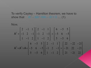
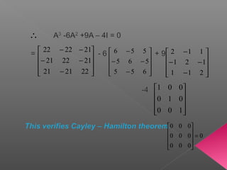
We are to prove that
pλ +p λ +p λ +...+p = 0
p A +p A +p A +...+p I= 0 ...(1)
I
⇒
n-1 n-2 n-3 -1
0 1 2 n-1 n
-1 n-1 n-2 n-3
0 1 2 n-1
n
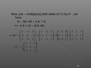
0 =p A +p A +p A +...+p +p A
1
A =- [p A +p A +p A +...+p I]
p](https://image.slidesharecdn.com/eigenvalueeigenvectorscaleyhamiltontheorem-151013075740-lva1-app6891/85/Eigen-value-eigen-vectors-caley-hamilton-theorem-34-320.jpg)


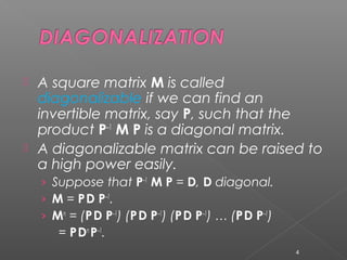
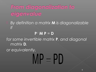
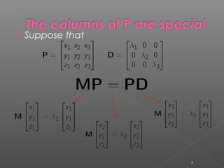
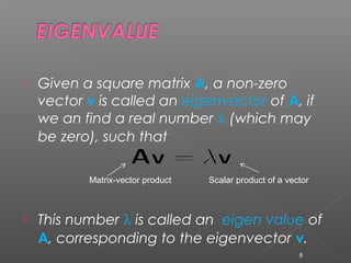
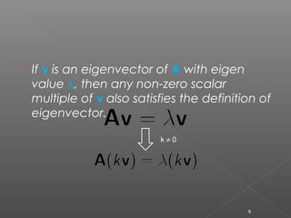
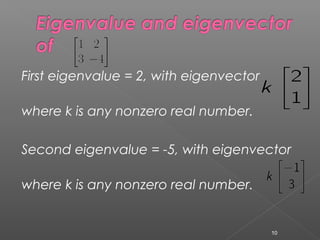
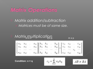
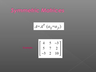
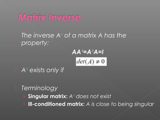
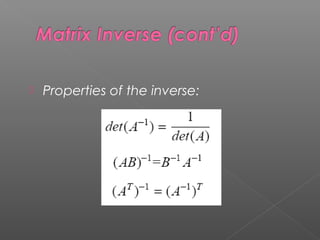
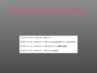
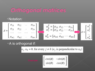
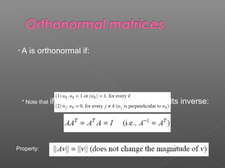
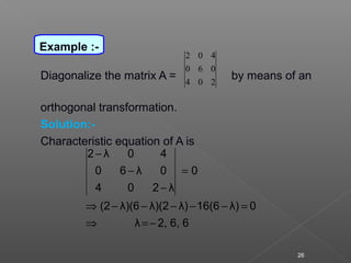
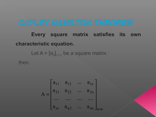
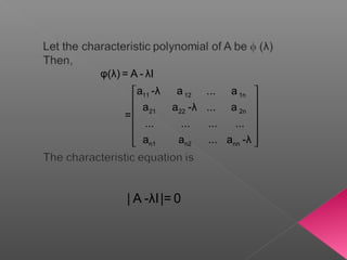
This document discusses several key linear algebra concepts: 1) A square matrix is diagonalizable if it can be transformed into a diagonal matrix through multiplication by an invertible matrix. Diagonalizable matrices can be easily raised to high powers. 2) Eigenvalues and eigenvectors are values and vectors that are unchanged by transformation by the matrix, up to a scaling factor for eigenvectors. 3) Orthogonal matrices preserve lengths and angles when multiplying vectors. The Cayley-Hamilton theorem states that every matrix satisfies its own characteristic equation.


