Downloaded 113 times


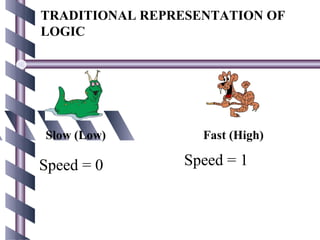
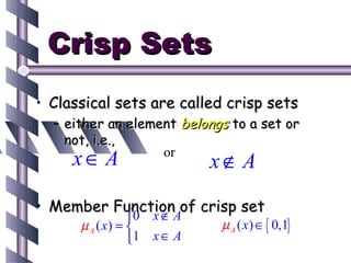
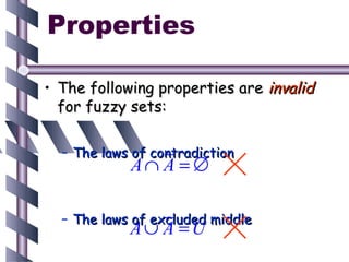
![FUZZY LOGIC
REPRESENTATION
Slowest
For every [ 0.0 – 0.25 ]
problem Slow
must [ 0.25 – 0.50 ]
represent in Fast
terms of [ 0.50 – 0.75 ]
fuzzy sets. Fastest
[ 0.75 – 1.00 ]](https://image.slidesharecdn.com/ghrcemaaimanojharsule-120812122051-phpapp01/85/Introduction-to-Artificial-Intelligence-6-320.jpg)
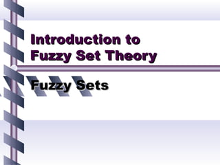
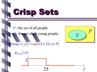
![Crisp sets µ A ( x) ∈ { 0,1}
Fuzzy Sets
µ A ( x) ∈ [0,1]
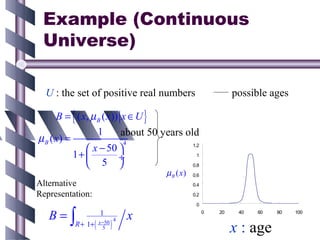
Example
µYoung ( y )
1
y](https://image.slidesharecdn.com/ghrcemaaimanojharsule-120812122051-phpapp01/85/Introduction-to-Artificial-Intelligence-12-320.jpg)
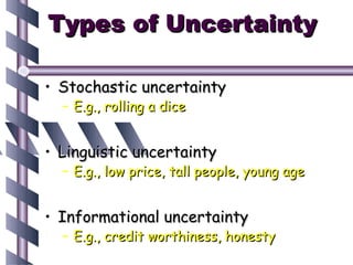
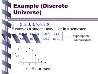
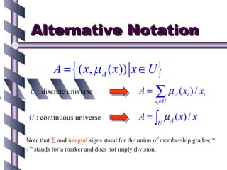
![Definition:
Fuzzy Sets and Membership
Functions
U : universe of discourse.
If U is a collection of objects denoted generically by x, then
a fuzzy set A in U is defined as a set of ordered pairs:
A = { ( x, µ A ( x)) x ∈ U }
membership
function
µ A : U → [0,1]](https://image.slidesharecdn.com/ghrcemaaimanojharsule-120812122051-phpapp01/85/Introduction-to-Artificial-Intelligence-13-320.jpg)
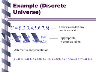

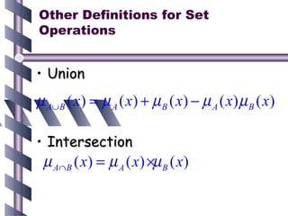
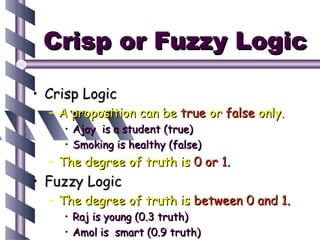
![T-Norm
Or called triangular norm.
T :[0,1] × [0,1] → [0,1]
1. Symmetry T ( x, y ) = T ( y , x )
2. Associativity T (T ( x, y ), z ) = T ( x, T ( y, z ))
3. Monotonicity x1 ≤ x2 , y1 ≤ y2 ⇒ T ( x1 , y1 ) ≤ T ( x2 , y2 )
4. Border Condition T ( x,1) = x](https://image.slidesharecdn.com/ghrcemaaimanojharsule-120812122051-phpapp01/85/Introduction-to-Artificial-Intelligence-28-320.jpg)
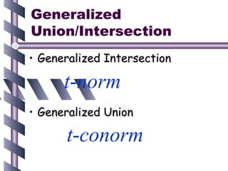
![T-Conorm Or called s-norm.
S :[0,1] × [0,1] → [0,1]
1. Symmetry S ( x, y ) = S ( y , x )
2. Associativity S ( S ( x, y ), z ) = S ( x, S ( y, z ))
3. Monotonicity x1 ≤ x2 , y1 ≤ y2 ⇒ S ( x1 , y1 ) ≤ S ( x2 , y2 )
4. Border Condition S ( x, 0) = x](https://image.slidesharecdn.com/ghrcemaaimanojharsule-120812122051-phpapp01/85/Introduction-to-Artificial-Intelligence-29-320.jpg)

![Dimension Expansion
Cylindrical Extension
A : a fuzzy set in X.
C(A) = [A↑X×Y] : cylindrical extension of A.
C ( A) = ∫ µ A ( x ) | ( x, y ) µC ( A ) ( x , y ) = µ A ( x )
X ×Y](https://image.slidesharecdn.com/ghrcemaaimanojharsule-120812122051-phpapp01/85/Introduction-to-Artificial-Intelligence-40-320.jpg)
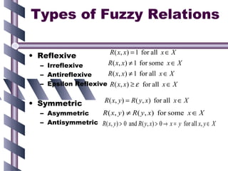
![Types of Fuzzy Relations
• Transitive (max-min transitive)
R ( x, z ) ≥ max min[ R ( x, y ), R ( y , z )] for all x,z ∈X
y∈Y
– Non-transitive:
For some (x,z), the above do not satisfy.
– Antitransitive:
R ( x, z ) < max min[ R ( x, y ), R ( y , z )] for all x,z ∈X
y∈Y
• Example: X = Set of cities, R=“very far”
Reflexive, symmetric, non-transitive](https://image.slidesharecdn.com/ghrcemaaimanojharsule-120812122051-phpapp01/85/Introduction-to-Artificial-Intelligence-42-320.jpg)
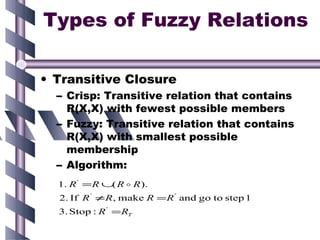
![Types of Fuzzy Relations
• Fuzzy Equivalence or Similarity
Relation
– Reflexive, symmetric, and transitive
– Decomposition:
R= ααR
⋅
α∈ ,1]
[0
α
R is a crisp equivalence relation.
Set of partitions :
∏ ={π(αR ) | α∈
(R) [0,1]}
– Partition Tree](https://image.slidesharecdn.com/ghrcemaaimanojharsule-120812122051-phpapp01/85/Introduction-to-Artificial-Intelligence-44-320.jpg)
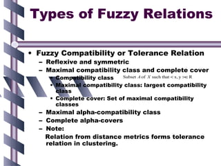


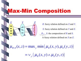
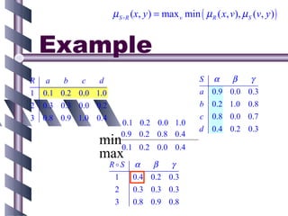
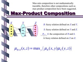
S: fuzzy relation defined on Y and Z. To find the composite relation R o S on X and Z: μR o S(x,z) = maxy [min(μR(x,y), μS(y,z))] For each x and z, find the maximum membership grade obtained by considering all possible y values and taking the minimum of the membership grades of R and S. This gives the generalized intersection-union definition of composition of fuzzy relations. It reduces to the usual composition rule when relations are crisp.