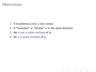
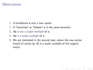
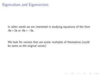
- There is a quiz tomorrow on sections 3.1 and 3.2 of the course material. Calculators will not be allowed and determinants must be calculated using the methods learned. - Eigenvalues and eigenvectors are related to the linear transformation of a matrix A acting on a vector x. They give a better understanding of the transformation. - The 1940 collapse of the Tacoma Narrows Bridge is explained by oscillations caused by the wind frequency matching the bridge's natural frequency, which is the eigenvalue of smallest magnitude based on a mathematical model of the bridge. Eigenvalues are important for engineering structure design.

1. Announcements
Quiz 3 tomorrow on sections 3.1 and 3.2
No calculators for this quiz. You have to nd the determinants
using the methods we have learned.

2. Section 5.1 Eigenvalues and Eigenvectors
Comes from the German word eigen meaning proper or
characteristic.
Gives a better understanding of the linear transformation x → Ax in
terms of elements that can be easily visualized.

3. Tacoma Narrows Bridge Collapse- 1940
1. Bridge forming small waves like a river

4. Tacoma Narrows Bridge Collapse- 1940
1. Bridge forming small waves like a river
2. Initially assumed safe but oscillations grew with time

5. Tacoma Narrows Bridge Collapse- 1940
1. Bridge forming small waves like a river
2. Initially assumed safe but oscillations grew with time
3. One edge of the road 28 ft higher than the other edge

6. Tacoma Narrows Bridge Collapse- 1940
1. Bridge forming small waves like a river
2. Initially assumed safe but oscillations grew with time
3. One edge of the road 28 ft higher than the other edge
4. Finally collapsed

7. Tacoma Narrows Bridge Collapse- 1940
Explanation:
1. Oscillation of bridge caused by the wind frequency being too
close to the natural frequency of the bridge

8. Tacoma Narrows Bridge Collapse- 1940
Explanation:
1. Oscillation of bridge caused by the wind frequency being too
close to the natural frequency of the bridge
2. Natural frequency of the bridge is the eigenvalue of the
smallest magnitude (based on a system that modeled the
bridge)

9. Tacoma Narrows Bridge Collapse- 1940
Explanation:
1. Oscillation of bridge caused by the wind frequency being too
close to the natural frequency of the bridge
2. Natural frequency of the bridge is the eigenvalue of the
smallest magnitude (based on a system that modeled the
bridge)
3. Eigenvalues are very important to engineers when they design
structures.

10. Electrical Systems
Radio Tuning
1. Trying to match the frequency with which your station is
broadcasting.
2. Eigenvalues were used during the radio design by engineers.

11. Cars
1. Use Eigenvalues to damp out noise for a quiet ride.

12. Cars
1. Use Eigenvalues to damp out noise for a quiet ride.
2. Also used in design of car stereo systems so that sounds create
listening pleasure
3. To reduce the vibration of the car due to the music.

13. Others
1. Test for cracks in a solid. (avoids testing each and every inch
of a beam for example)

14. Others
1. Test for cracks in a solid. (avoids testing each and every inch
of a beam for example)
2. Used by oil companies to explore land for oil.

15. Others
1. Test for cracks in a solid. (avoids testing each and every inch
of a beam for example)
2. Used by oil companies to explore land for oil.
3. Applications in economics, physics, chemistry, biology (red
blood cell production)

16. Others
1. Test for cracks in a solid. (avoids testing each and every inch
of a beam for example)
2. Used by oil companies to explore land for oil.
3. Applications in economics, physics, chemistry, biology (red
blood cell production)
4. Discrete (and continuous) linear dynamical systems (part of
MA3521)

17. Others
1. Test for cracks in a solid. (avoids testing each and every inch
of a beam for example)
2. Used by oil companies to explore land for oil.
3. Applications in economics, physics, chemistry, biology (red
blood cell production)
4. Discrete (and continuous) linear dynamical systems (part of
MA3521)
5. Pure and Applied Mathematics

18. Back to matrix-vector product
3 −2 −1
Let A = . Find Au and Av where u = and
1 0 −2
2
v= (the image of u and v after being acted on by A.)
1

19. Back to matrix-vector product
3 −2 −1
Let A = . Find Au and Av where u = and
1 0 −2
2
v= (the image of u and v after being acted on by A.)
1
3 −2 −1 −3 + 4 1
A u= = =
1 0 −2 −1 − 0 −1
3 −2 2 6−2 4
A v= = = = 2v
1 0 1 2+0 2

20. y
x
0

21. y
x
0
u

22. y
x
0
A u
u

23. y
x
0
A u
u

24. y
v
x
0
A u
u

25. y
A v
v
x
0
A u
u

26. y
A v
v
x
0
A u
u

27. Observations
1. A transforms u into a new vector.

28. Observations
1. A transforms u into a new vector.
2. A stretches or dilates v in the same direction.

29. Observations
1. A transforms u into a new vector.
2. A stretches or dilates v in the same direction.
3. Au is not a scalar multiple of u

30. Observations
1. A transforms u into a new vector.
2. A stretches or dilates v in the same direction.
3. Au is not a scalar multiple of u
4. Av is a scalar multiple of v

31. Observations
1. A transforms u into a new vector.
2. A stretches or dilates v in the same direction.
3. Au is not a scalar multiple of u
4. Av is a scalar multiple of v
5. We are interested in the second case, where the new vector
(result of action by A) is a scalar multiple of the original
vector.

32. Eigenvalues and Eigenvectors
In other words we are interested in studying equations of the form
Ax = 2x or Ax = −3x.
We look for vectors that are scalar multiples of themselves (could
be same as the original vector)

33. Eigenvalues and Eigenvectors
Denition
An eigenvector of an n × n matrix A is a NON-ZERO vector x
such that Ax = λx for some scalar λ.
A scalar λ is called an eigenvalue of A if there is a nontrivial (or
nonzero) solution x to Ax = λx; such an x is called an eigenvector
corresponding to λ.

34. Why nonzero?
Go back to Ax = λx. What is an obvious solution to this equation?

35. Why nonzero?
Go back to Ax = λx. What is an obvious solution to this equation?
We know that A0 = λ0 always. There is nothing interesting about
the zero (or the trivial) solution. So we need a nonzero vector for
eigenvector.

36. Why nonzero?
Go back to Ax = λx. What is an obvious solution to this equation?
We know that A0 = λ0 always. There is nothing interesting about
the zero (or the trivial) solution. So we need a nonzero vector for
eigenvector.
An eigenvalue can be zero. (We will come back to this case later)

37. Example
7 2 1 1
Let A = . Check whether u = and v = are
−4 1 −1 −3
eigenvectors of A. If yes, nd the corresponding eigenvalues.

38. Example
7 2 1 1
Let A = . Check whether u = and v = are
−4 1 −1 −3
eigenvectors of A. If yes, nd the corresponding eigenvalues.
Solution: To check whether a given vector u or v is an eigenvector
of A is easy.
Find the product Au and check whether the new vector is a scalar
multiple of u. Also nd Av and check whether the new vector is a
scalar multiple of v.

39. Example
7 2 1 1
Let A = . Check whether u = and v = are
−4 1 −1 −3
eigenvectors of A. If yes, nd the corresponding eigenvalues.
Solution: To check whether a given vector u or v is an eigenvector
of A is easy.
Find the product Au and check whether the new vector is a scalar
multiple of u. Also nd Av and check whether the new vector is a
scalar multiple of v.
7 2 1 5
A u= = = 5u
−4 1 −1 −5
7 2 1 1
A v= = = λv
−4 1 −3 −7

40. Example
7 2 1 1
Let A = . Check whether u = and v = are
−4 1 −1 −3
eigenvectors of A. If yes, nd the corresponding eigenvalues.
Solution: To check whether a given vector u or v is an eigenvector
of A is easy.
Find the product Au and check whether the new vector is a scalar
multiple of u. Also nd Av and check whether the new vector is a
scalar multiple of v.
7 2 1 5
A u= = = 5u
−4 1 −1 −5
7 2 1 1
A v= = = λv
−4 1 −3 −7
So u is an eigenvector with λ = 5 and v is not an eigenvector.

41. Example
7 2
Let A = . Show that 3 is an eigenvalue of A and nd the
−4 1
corresponding eigenvectors.
Solution: 3 is an eigenvalue of A if and only if the equation Ax = 3x
has a nontrivial solution.

42. Example
7 2
Let A = . Show that 3 is an eigenvalue of A and nd the
−4 1
corresponding eigenvectors.
Solution: 3 is an eigenvalue of A if and only if the equation Ax = 3x
has a nontrivial solution. This means
A x − 3x = 0
has a nontrivial solution. Or
(A − 3I )x = 0
Back to homogeneous systems, trivial and nontrivial solutions.

43. Revisiting Homogeneous Systems
1. Zero is always a solution (trivial solution).
2. For nontrivial solutions, we need linearly dependent columns

44. Revisiting Homogeneous Systems
1. Zero is always a solution (trivial solution).
2. For nontrivial solutions, we need linearly dependent columns
3. This means there are nonpivot columns or free variables

45. Revisiting Homogeneous Systems
1. Zero is always a solution (trivial solution).
2. For nontrivial solutions, we need linearly dependent columns
3. This means there are nonpivot columns or free variables
4. The free variables lead us to nontrivial solutions.

46. Example
Write the matrix
7 2 3 0 4 2
A − 3I = − = .
−4 1 0 3 −4 −2
What do you think about the columns? Linearly dep/indep?

47. Example
Write the matrix
7 2 3 0 4 2
A − 3I = − = .
−4 1 0 3 −4 −2
What do you think about the columns? Linearly dep/indep?They
are linearly dependent. So the homogeneous system has

48. Example
Write the matrix
7 2 3 0 4 2
A − 3I = − = .
−4 1 0 3 −4 −2
What do you think about the columns? Linearly dep/indep?They
are linearly dependent. So the homogeneous system has nontrivial
solutions. Thus 3 is an eigenvalue of A.

49. Example
We still have to nd the eigenvectors for this eigenvalue (λ = 3).
Start with the matrix A − 3I and do row operations.
 
 4 2 0
R1+R2

 
 
−4 −2 0
 
 
 4 2 0 
 
 
0 0 0
 

50. Example
We still have to nd the eigenvectors for this eigenvalue (λ = 3).
Start with the matrix A − 3I and do row operations.
 
 4 2 0
R1+R2

 
 
−4 −2 0
 
 
 4 2 0 
 
 
0 0 0
 
So, 4x1 = −2x2 where x2 is free. Or, x1 = − 1 x2 .
2

51. Example
We still have to nd the eigenvectors for this eigenvalue (λ = 3).
Start with the matrix A − 3I and do row operations.
 
 4 2 0
R1+R2

 
 
−4 −2 0
 
 
 4 2 0 
 
 
0 0 0
 
So, 4x1 = −2x2 where x2 is free. Or, x1 = − 1 x2 . Our solution is
2
thus,
x1 − 1 x2
2 −1
2
= = x2 .
x2 x2 1

52. Example
Choose any value for x2 other than zero. Preferably, choose
something that will clear the fraction. So choose x2 = 2.

53. Example
Choose any value for x2 other than zero. Preferably, choose
something that will clear the fraction. So choose x2 = 2. This gives,
x1 −1
2 −1
=2 = .
x2 1 2
Remember that this is an eigenvector of A. Depending on your
−1
2
choice of x2 , any scalar multiple of is an eigenvector of A.
1

54. Notes
1. Echelon form is used to nd eigenvectors BUT NOT
eigenvalues.

55. Notes
1. Echelon form is used to nd eigenvectors BUT NOT
eigenvalues.
2. λ is an eigenvalue of A if and only if the equation
(A − λI )x = 0 has nontrivial solution.

56. Notes
1. Echelon form is used to nd eigenvectors BUT NOT
eigenvalues.
2. λ is an eigenvalue of A if and only if the equation
(A − λI )x = 0 has nontrivial solution.
3. All solutions to (A − λI )x = 0 is nothing but the Null Space of
(A − λI ).

57. Notes
1. Echelon form is used to nd eigenvectors BUT NOT
eigenvalues.
2. λ is an eigenvalue of A if and only if the equation
(A − λI )x = 0 has nontrivial solution.
3. All solutions to (A − λI )x = 0 is nothing but the Null Space of
(A − λI ).
4. This set is a subspace of Rn and is called the eigenspace of A
corresponding to λ.

58. Notes
1. Echelon form is used to nd eigenvectors BUT NOT
eigenvalues.
2. λ is an eigenvalue of A if and only if the equation
(A − λI )x = 0 has nontrivial solution.
3. All solutions to (A − λI )x = 0 is nothing but the Null Space of
(A − λI ).
4. This set is a subspace of Rn and is called the eigenspace of A
corresponding to λ.
5. Eigenspace consists of the zero vector and all eigenvectors
corresponding to λ.

59. Steps to check if λ is an eigenvalue
1. Write the matrix A − λI

60. Steps to check if λ is an eigenvalue
1. Write the matrix A − λI
2. Check whether the columns are linearly dependent (existence
of free variables)

61. Steps to check if λ is an eigenvalue
1. Write the matrix A − λI
2. Check whether the columns are linearly dependent (existence
of free variables)
3. If the columns are linearly dependent, λ is an eigenvalue.

62. Steps to nd the eigenvectors for λ
Once we have an eigenvalue λ,
1. Start with the matrix A − λI

63. Steps to nd the eigenvectors for λ
Once we have an eigenvalue λ,
1. Start with the matrix A − λI
2. Row reduce to echelon form to identify the basic and free
variables.

64. Steps to nd the eigenvectors for λ
Once we have an eigenvalue λ,
1. Start with the matrix A − λI
2. Row reduce to echelon form to identify the basic and free
variables.
3. Express the basic variables in terms of free variables, write the
answer in vector form.

65. Steps to nd the eigenvectors for λ
Once we have an eigenvalue λ,
1. Start with the matrix A − λI
2. Row reduce to echelon form to identify the basic and free
variables.
3. Express the basic variables in terms of free variables, write the
answer in vector form.
4. Choose a convenient value for the free variable (NEVER
choose zero).

66. Example 6, section 5.1
1 3 6 7
   
Is  −2  an eigenvector of A= 3 3 7 . If yes, nd the
1 5 6 5
corresponding eigenvalue.

67. Example 6, section 5.1
1 3 6 7
   
Is  −2  an eigenvector of A= 3 3 7 . If yes, nd the
1 5 6 5
corresponding eigenvalue.
Solution:
3 6 7 1 3 − 12 + 7 −2
      
 3 3 7   −2  =  3 − 6 + 7  =  4 
5 6 5 1 5 − 12 + 5 −2

68. Example 6, section 5.1
1 3 6 7
   
Is  −2  an eigenvector of A= 3 3 7 . If yes, nd the
1 5 6 5
corresponding eigenvalue.
Solution:
3 6 7 1 3 − 12 + 7 −2
      
 3 3 7   −2  =  3 − 6 + 7  =  4 
5 6 5 1 5 − 12 + 5 −2
1
 
The new vector is -2 times the old vector. So  −2  is an
1
eigenvector of A with eigenvalue λ = −2.

69. Example 8, section 5.1
1 2 2
 
Is λ = 3 an eigenvalue of A =  3 −2 1 ? If yes, nd the
0 1 1
corresponding eigenvector.

70. Example 8, section 5.1
1 2 2
 
Is λ = 3 an eigenvalue of A =  3 −2 1 ? If yes, nd the
0 1 1
corresponding eigenvector.
Solution:
1 2 2 3 0 0 −2 2 2
     
A − 3I =  3 −2 1  −  0 3 0  =  3 −5 1 
0 1 1 0 0 3 0 1 −2

71. Example 8, section 5.1
1 2 2
 
Is λ = 3 an eigenvalue of A =  3 −2 1 ? If yes, nd the
0 1 1
corresponding eigenvector.
Solution:
1 2 2 3 0 0 −2 2 2
     
A − 3I =  3 −2 1  −  0 3 0  =  3 −5 1 
0 1 1 0 0 3 0 1 −2
How to know whether the columns are linearly dependent? You can
check whether the determinant of this matrix is zero. (Or you could
row reduce and check if there are free variables)

72. Example 8, section 5.1
1 2 2
 
Is λ = 3 an eigenvalue of A =  3 −2 1 ? If yes, nd the
0 1 1
corresponding eigenvector.
Solution:
1 2 2 3 0 0 −2 2 2
     
A − 3I =  3 −2 1  −  0 3 0  =  3 −5 1 
0 1 1 0 0 3 0 1 −2
How to know whether the columns are linearly dependent? You can
check whether the determinant of this matrix is zero. (Or you could
row reduce and check if there are free variables)
If det(A − 3I ) = 0, that means A − 3I has linearly dependent columns
(or there is a nontrivial solution).

73. Example 8, section 5.1
1 2 2
 
Is λ = 3 an eigenvalue of A =  3 −2 1 ? If yes, nd the
0 1 1
corresponding eigenvector.
Solution:
1 2 2 3 0 0 −2 2 2
     
A − 3I =  3 −2 1  −  0 3 0  =  3 −5 1 
0 1 1 0 0 3 0 1 −2
How to know whether the columns are linearly dependent? You can
check whether the determinant of this matrix is zero. (Or you could
row reduce and check if there are free variables)
If det(A − 3I ) = 0, that means A − 3I has linearly dependent columns
(or there is a nontrivial solution).
Here det(A − 3I ) = 0 (Do this yourself), so the columns are linearly
dependent and so λ = 3 is an eigenvalue.

74. To nd an eigenvector, start with A − 3I and row reduce
−2 2 2
 
A − 3I =  3 −5 1 
0 1 −2
Divide R1 by -2 and we get
1 −1 −1
 
A − 3I =  3 −5 1 
0 1 −2
 
 1 −1 −1 0
R2-3R1

 
 
 3 −5 1 0
 

 
 
 
0 1 −2 0

75.  
 1 −1 −1 0 
 
 
 0 −2 4 0
 
R3+0.5R2

 
 
 
0 1 −2 0
1 −1 −1 0
 
 0 −2 4 0 
0 0 0 0
We have x2 = 2x3 and x1 = x2 + x3 = 3x3 .Our solution is thus,
3x3 3
     
x1
 x2  =  2x3  = x3  2  .
x3 x3 1
Choose x3 = 1 and we have
3
   
x1
 x2  =  2 .
x3 1

76. Example 12, section 5.1
7 4
Find a basis for the eigenspace of A = corresponding to
−3 −1
λ = 1, 5.

77. Example 12, section 5.1
7 4
Find a basis for the eigenspace of A = corresponding to
−3 −1
λ = 1, 5.
Solution: For λ = 1,
7 4 1 0 6 4
A −I = − =
−3 −1 0 1 −3 −2

78. Example 12, section 5.1
7 4
Find a basis for the eigenspace of A = corresponding to
−3 −1
λ = 1, 5.
Solution: For λ = 1,
7 4 1 0 6 4
A −I = − =
−3 −1 0 1 −3 −2
 
 6 4 0
R2+0.5R1

 
 
−3 −2 0
 
 
 6 4 0 
 
 
0 0 0
 

79. Example 12, section 5.1
From the rst row, 6x1 = −4x2 or x1 = − 2 x2 .
3

80. Example 12, section 5.1
From the rst row, 6x1 = −4x2 or x1 = − 2 x2 . Our solution is thus,
3
x1 − 2 x2
3 −2
3
= = x2 .
x2 x2 1

81. Example 12, section 5.1
From the rst row, 6x1 = −4x2 or x1 = − 2 x2 . Our solution is thus,
3
x1 − 2 x2
3 −2
3
= = x2 .
x2 x2 1
Choose a convenient value for x2 . Pick x2 = 3 to clear the fraction.
This gives
x1 −2
3 −2
=3 = .
x2 1 3

82. Example 12, section 5.1
For λ = 5,
7 4 5 0 2 4
A − 5I = − =
−3 −1 0 5 −3 −6

83. Example 12, section 5.1
For λ = 5,
7 4 5 0 2 4
A − 5I = − =
−3 −1 0 5 −3 −6
Divide R1 by 2 and we get
1 2
−3 −6

84. Example 12, section 5.1
For λ = 5,
7 4 5 0 2 4
A − 5I = − =
−3 −1 0 5 −3 −6
Divide R1 by 2 and we get
1 2
−3 −6
 
 1 2 0
R2+3R1

 
 
−3 −6 0
 
 
 1 2 0 
 
 
0 0 0
 

85. Example 12, section 5.1
From the rst row, x1 = −2x2 . Our solution is thus,

86. Example 12, section 5.1
From the rst row, x1 = −2x2 . Our solution is thus,
x1 −2x2 −2
= = x2 .
x2 x2 1

87. Example 12, section 5.1
From the rst row, x1 = −2x2 . Our solution is thus,
x1 −2x2 −2
= = x2 .
x2 x2 1
Choose a convenient value for x2 . Pick x2 = 1. This gives
x1 −2
= .
x2 1

88. Example 14, section 5.1
1 0 −1
 
Find a basis for the eigenspace of A =  1 −3 0 
4 −13 1
corresponding to λ = −2.
Solution: For λ = −2,
1 0 −1 2 0 0 3 0 −1
     
A + 2I =  1 −3 0  +  0 2 0  =  1 −1 0 
4 −13 1 0 0 2 4 −13 3

89. Example 14, section 5.1
1 0 −1
 
Find a basis for the eigenspace of A =  1 −3 0 
4 −13 1
corresponding to λ = −2.
Solution: For λ = −2,
1 0 −1 2 0 0 3 0 −1
     
A + 2I =  1 −3 0  +  0 2 0  =  1 −1 0 
4 −13 1 0 0 2 4 −13 3
 
 3 0 −1 0
Swap

 
 
 1 −1 0 0
 

 
 
 
4 −13 3 0

90.  
 1 −1 0 0
R2-3R1

R3-4R1
 
 
 3 0 −1 0
 

 
 
 
4 −13 3 0

91.  
 1 −1 0 0
R2-3R1

R3-4R1
 
 
 3 0 −1 0
 

 
 
 
4 −13 3 0
 
 1 −1 0 0 
 
 
 0 3 −1 0
 
R3+3R2

 
 
 
0 −9 3 0

92. Example 14, section 5.1
1 −1 0 0
 
 0 3 −1 0 
0 0 0 0

93. Example 14, section 5.1
1 −1 0 0
 
 0 3 −1 0 
0 0 0 0
Here x3 is a free variable.
From the second row, 3x2 = x3 or x2 = 1 x3 .
3
From rst row, x1 = x2 and so x1 = 1 x3 .
3

94. Example 14, section 5.1
1 −1 0 0
 
 0 3 −1 0 
0 0 0 0
Here x3 is a free variable.
From the second row, 3x2 = x3 or x2 = 1 x3 .
3
From rst row, x1 = x2 and so x1 = 1 x3 .
3
Our solution is thus,
   1   1 
x1
3 3 x
3
 x2  =  1 x3  = x3  1  .
3 3
x3 x3 1

95. Example 14, section 5.1
1 −1 0 0
 
 0 3 −1 0 
0 0 0 0
Here x3 is a free variable.
From the second row, 3x2 = x3 or x2 = 1 x3 .
3
From rst row, x1 = x2 and so x1 = 1 x3 .
3
Our solution is thus,
   1   1 
x1
3 3 x
3
 x2  =  1 x3  = x3  1  .
3 3
x3 x3 1
Choose x3 = 3 and we have
1
   
x1
 x2  =  1 .
x3 3

96. Any Surprises to Expect?
Try problems 13 and 15 in your homework. There might be
something interesting going on in these cases. If you get stuck, we
will go over them in class tomorrow.

97. Triangular Matrices
Theorem
The eigenvalues of a triangular matrix are the entries on its main
diagonal.

98. Triangular Matrices
Theorem
The eigenvalues of a triangular matrix are the entries on its main
diagonal.
Proof.
For simplicity, consider a 3 × 3 upper triangular matrix. Then
0 0
λ −λ
     
a11 a12 a13 a11 a12 a13
A −λI =  0 a22 a23 − 0 λ 0  =  0 a22 −λ a23 
0 0 a33 0 0 λ 0 0 a33 −λ
(A − λI )x = 0 has a free variable if and only if atleast one of the
diagonal entries is zero. This happens if and only if λ equals one of
the entries a11 , a22 , a33 of A.

99. Triangular Matrices
Example
1. Let
5 1 9
 
A=  0 2 3 
0 0 6
The eigenvalues of A are 5, 2 and 6.

100. Triangular Matrices
Example
1. Let
5 1 9
 
A=  0 2 3 
0 0 6
The eigenvalues of A are 5, 2 and 6.
2. Let
4 1 9
 
A= 0 0 3 
0 0 6
The eigenvalues of A are 4, 0 and 6.