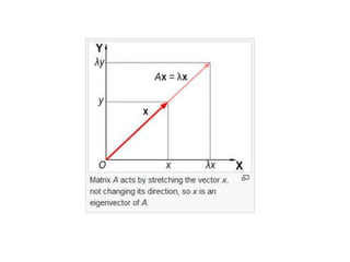
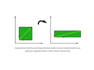
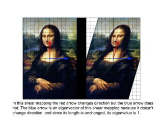
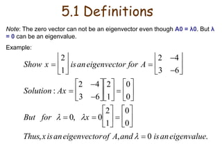
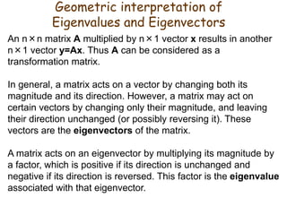
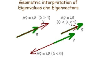
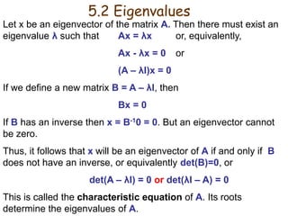
Chapter 6 – Part 1
Eigenvalues and Eigenvectors
In this shear mapping the red arrow changes direction but the blue arrow does
not. The blue arrow is an eigenvector of this shear mapping because it doesn't
change direction, and since its length is unchanged, its eigenvalue is 1.
5.1 Definitions
Definition 1: A nonzero vector x is an eigenvector (or characteristic vector)
of a square matrix A if there exists a scalar λ such that Ax = λx. Then λ is an
eigenvalue (or characteristic value) of A.
Example:
.
3
and
an
is
Thus
3
0
1
3
0
3
0
1
2
0
0
3
:
2
0
0
3
0
1
eigenvalue
an
is
r
eigenvecto
x
x
x
Ax
Solution
A
for
r
eigenvecto
an
is
x
Show













































5.1 Definitions
Note: The zero vector can not be an eigenvector even though A0 = λ0. But λ
= 0 can be an eigenvalue.
Example:
Show x 
2
1





isaneigenvector for A 
2 4
3 6






Solution : Ax 
2 4
3 6






2
1






0
0






But for   0, x  0
2
1






0
0






Thus,xisaneigenvectorof A,and   0 isaneigenvalue.
Geometric interpretation of
Eigenvalues and Eigenvectors
An n×n matrix A multiplied by n×1 vector x results in another
n×1 vector y=Ax. Thus A can be considered as a
transformation matrix.
In general, a matrix acts on a vector by changing both its
magnitude and its direction. However, a matrix may act on
certain vectors by changing only their magnitude, and leaving
their direction unchanged (or possibly reversing it). These
vectors are the eigenvectors of the matrix.
A matrix acts on an eigenvector by multiplying its magnitude by
a factor, which is positive if its direction is unchanged and
negative if its direction is reversed. This factor is the eigenvalue
associated with that eigenvector.
Geometric interpretation of
Eigenvalues and Eigenvectors
5.2 Eigenvalues
Let x be an eigenvector of the matrix A. Then there must exist an
eigenvalue λ such that Ax = λx or, equivalently,
Ax - λx = 0 or
(A – λI)x = 0
If we define a new matrix B = A – λI, then
Bx = 0
If B has an inverse then x = B-10 = 0. But an eigenvector cannot
be zero.
Thus, it follows that x will be an eigenvector of A if and only if B
does not have an inverse, or equivalently det(B)=0, or
det(A – λI) = 0 or det(λI – A) = 0
This is called the characteristic equation of A. Its roots
determine the eigenvalues of A.
Example 1: Find the eigenvalues of
two eigenvalues: 1,  2
Note: The roots of the characteristic equation can be repeated. That is, λ1 = λ2
=…= λk. If that happens, the eigenvalue is said to be of multiplicity k.
Example 2: Find the eigenvalues of
λ = 2 is an eigenvalue of multiplicity 3.









5
1
12
2
A
0
)
2
)(
1
(
2
3
12
)
5
)(
2
(
5
1
12
2
2
























 A
I
5.2 Eigenvalues: examples











2
0
0
0
2
0
0
1
2
A
0
)
2
(
2
0
0
0
2
0
0
1
2
3








 



 A
I
Example 1 (cont.):





 














0
0
4
1
4
1
12
3
)
1
(
:
1 A
I

0
,
1
4
,
4
0
4
2
1
1
2
1
2
1




















t
t
x
x
t
x
t
x
x
x
x





 














0
0
3
1
3
1
12
4
)
2
(
:
2 A
I

0
,
1
3
2
1
2 













 s
s
x
x
x
5.3 Eigenvectors
To each distinct eigenvalue of a matrix A there will correspond at least one
eigenvector which can be found by solving the appropriate set of homogenous
equations. If λi is an eigenvalue then the corresponding eigenvector xi is the
solution of (λiI – A)xi = 0
ERO
ERO
Example 2 (cont.): Find the eigenvectors of
Recall that λ = 2 is an eigenvector of multiplicity 3.
Solve the homogeneous linear system represented by
Let . The eigenvectors of  = 2 are of the
form
s and t not both zero.






























 


0
0
0
0
0
0
0
0
0
0
1
0
)
2
(
3
2
1
x
x
x
A
I x
t
x
s
x 
 3
1 ,
,
1
0
0
0
0
1
0
3
2
1











































 t
s
t
s
x
x
x
x
5.3 Eigenvectors











2
0
0
0
2
0
0
1
2
A
5.4 Properties of Eigenvalues and Eigenvectors
Definition: The trace of a matrix A, designated by tr(A), is the sum
of the elements on the main diagonal.
Property 1: The sum of the eigenvalues of a matrix equals the
trace of the matrix.
Property 2: A matrix is singular if and only if it has a zero
eigenvalue.
Property 3: The eigenvalues of an upper (or lower) triangular
matrix are the elements on the main diagonal.
Property 4: If λ is an eigenvalue of A and A is invertible, then 1/λ
is an eigenvalue of matrix A-1.
5.4 Properties of Eigenvalues and
Eigenvectors
Property 5: If λ is an eigenvalue of A then kλ is an eigenvalue of
kA where k is any arbitrary scalar.
Property 6: If λ is an eigenvalue of A then λk is an eigenvalue of
Ak for any positive integer k.
Property 8: If λ is an eigenvalue of A then λ is an eigenvalue of AT.
Property 9: The product of the eigenvalues of a matrix equals the
determinant of the matrix.

Lecture_06_Part_1.ppt

  • 1.
    Chapter 6 –Part 1 Eigenvalues and Eigenvectors
  • 4.
    In this shearmapping the red arrow changes direction but the blue arrow does not. The blue arrow is an eigenvector of this shear mapping because it doesn't change direction, and since its length is unchanged, its eigenvalue is 1.
  • 5.
    5.1 Definitions Definition 1:A nonzero vector x is an eigenvector (or characteristic vector) of a square matrix A if there exists a scalar λ such that Ax = λx. Then λ is an eigenvalue (or characteristic value) of A. Example: . 3 and an is Thus 3 0 1 3 0 3 0 1 2 0 0 3 : 2 0 0 3 0 1 eigenvalue an is r eigenvecto x x x Ax Solution A for r eigenvecto an is x Show                                             
  • 6.
    5.1 Definitions Note: Thezero vector can not be an eigenvector even though A0 = λ0. But λ = 0 can be an eigenvalue. Example: Show x  2 1      isaneigenvector for A  2 4 3 6       Solution : Ax  2 4 3 6       2 1       0 0       But for   0, x  0 2 1       0 0       Thus,xisaneigenvectorof A,and   0 isaneigenvalue.
  • 7.
    Geometric interpretation of Eigenvaluesand Eigenvectors An n×n matrix A multiplied by n×1 vector x results in another n×1 vector y=Ax. Thus A can be considered as a transformation matrix. In general, a matrix acts on a vector by changing both its magnitude and its direction. However, a matrix may act on certain vectors by changing only their magnitude, and leaving their direction unchanged (or possibly reversing it). These vectors are the eigenvectors of the matrix. A matrix acts on an eigenvector by multiplying its magnitude by a factor, which is positive if its direction is unchanged and negative if its direction is reversed. This factor is the eigenvalue associated with that eigenvector.
  • 8.
  • 9.
    5.2 Eigenvalues Let xbe an eigenvector of the matrix A. Then there must exist an eigenvalue λ such that Ax = λx or, equivalently, Ax - λx = 0 or (A – λI)x = 0 If we define a new matrix B = A – λI, then Bx = 0 If B has an inverse then x = B-10 = 0. But an eigenvector cannot be zero. Thus, it follows that x will be an eigenvector of A if and only if B does not have an inverse, or equivalently det(B)=0, or det(A – λI) = 0 or det(λI – A) = 0 This is called the characteristic equation of A. Its roots determine the eigenvalues of A.
  • 10.
    Example 1: Findthe eigenvalues of two eigenvalues: 1,  2 Note: The roots of the characteristic equation can be repeated. That is, λ1 = λ2 =…= λk. If that happens, the eigenvalue is said to be of multiplicity k. Example 2: Find the eigenvalues of λ = 2 is an eigenvalue of multiplicity 3.          5 1 12 2 A 0 ) 2 )( 1 ( 2 3 12 ) 5 )( 2 ( 5 1 12 2 2                          A I 5.2 Eigenvalues: examples            2 0 0 0 2 0 0 1 2 A 0 ) 2 ( 2 0 0 0 2 0 0 1 2 3               A I
  • 11.
    Example 1 (cont.):                     0 0 4 1 4 1 12 3 ) 1 ( : 1 A I  0 , 1 4 , 4 0 4 2 1 1 2 1 2 1                     t t x x t x t x x x x                      0 0 3 1 3 1 12 4 ) 2 ( : 2 A I  0 , 1 3 2 1 2                s s x x x 5.3 Eigenvectors To each distinct eigenvalue of a matrix A there will correspond at least one eigenvector which can be found by solving the appropriate set of homogenous equations. If λi is an eigenvalue then the corresponding eigenvector xi is the solution of (λiI – A)xi = 0 ERO ERO
  • 12.
    Example 2 (cont.):Find the eigenvectors of Recall that λ = 2 is an eigenvector of multiplicity 3. Solve the homogeneous linear system represented by Let . The eigenvectors of  = 2 are of the form s and t not both zero.                                   0 0 0 0 0 0 0 0 0 0 1 0 ) 2 ( 3 2 1 x x x A I x t x s x   3 1 , , 1 0 0 0 0 1 0 3 2 1                                             t s t s x x x x 5.3 Eigenvectors            2 0 0 0 2 0 0 1 2 A
  • 13.
    5.4 Properties ofEigenvalues and Eigenvectors Definition: The trace of a matrix A, designated by tr(A), is the sum of the elements on the main diagonal. Property 1: The sum of the eigenvalues of a matrix equals the trace of the matrix. Property 2: A matrix is singular if and only if it has a zero eigenvalue. Property 3: The eigenvalues of an upper (or lower) triangular matrix are the elements on the main diagonal. Property 4: If λ is an eigenvalue of A and A is invertible, then 1/λ is an eigenvalue of matrix A-1.
  • 14.
    5.4 Properties ofEigenvalues and Eigenvectors Property 5: If λ is an eigenvalue of A then kλ is an eigenvalue of kA where k is any arbitrary scalar. Property 6: If λ is an eigenvalue of A then λk is an eigenvalue of Ak for any positive integer k. Property 8: If λ is an eigenvalue of A then λ is an eigenvalue of AT. Property 9: The product of the eigenvalues of a matrix equals the determinant of the matrix.