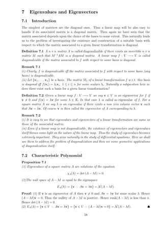
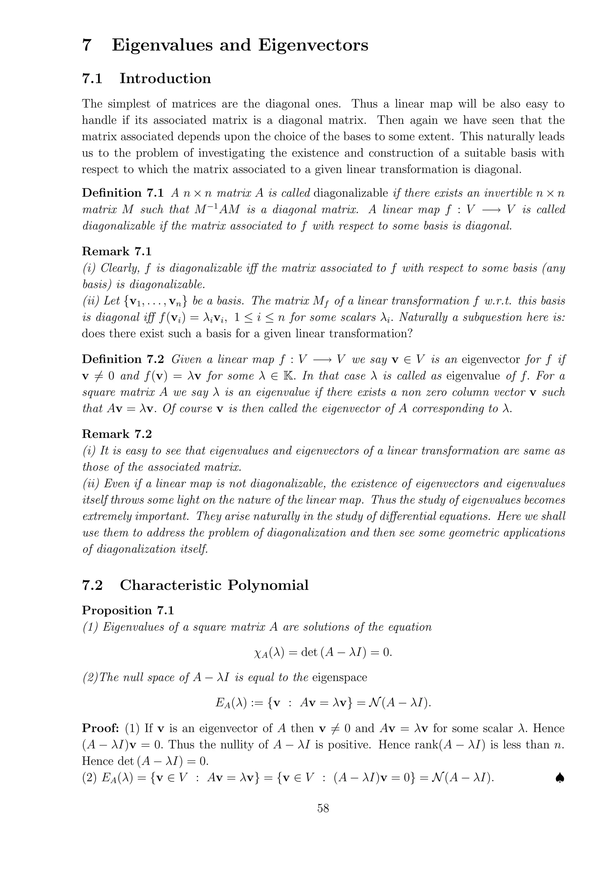
The document discusses eigenvalues and eigenvectors of linear transformations and matrices. It begins by defining a diagonalizable matrix as one that can be transformed into a diagonal matrix through a change of basis. It then defines eigenvalues and eigenvectors for both linear transformations and matrices. The characteristic polynomial of a matrix is introduced, which has roots that are the eigenvalues of the matrix. It is shown that the algebraic multiplicity of an eigenvalue is equal to its multiplicity as a root of the characteristic polynomial, while the geometric multiplicity is the dimension of the eigenspace. The algebraic multiplicity is always greater than or equal to the geometric multiplicity.

1. 7 Eigenvalues and Eigenvectors
7.1 Introduction
The simplest of matrices are the diagonal ones. Thus a linear map will be also easy to
handle if its associated matrix is a diagonal matrix. Then again we have seen that the
matrix associated depends upon the choice of the bases to some extent. This naturally leads
us to the problem of investigating the existence and construction of a suitable basis with
respect to which the matrix associated to a given linear transformation is diagonal.
Definition 7.1 A n × n matrix A is called diagonalizable if there exists an invertible n × n
matrix M such that M−1
AM is a diagonal matrix. A linear map f : V −→ V is called
diagonalizable if the matrix associated to f with respect to some basis is diagonal.
Remark 7.1
(i) Clearly, f is diagonalizable iff the matrix associated to f with respect to some basis (any
basis) is diagonalizable.
(ii) Let {v1, . . . , vn} be a basis. The matrix Mf of a linear transformation f w.r.t. this basis
is diagonal iff f(vi) = λivi, 1 ≤ i ≤ n for some scalars λi. Naturally a subquestion here is:
does there exist such a basis for a given linear transformation?
Definition 7.2 Given a linear map f : V −→ V we say v ∈ V is an eigenvector for f if
v 6= 0 and f(v) = λv for some λ ∈ K. In that case λ is called as eigenvalue of f. For a
square matrix A we say λ is an eigenvalue if there exists a non zero column vector v such
that Av = λv. Of course v is then called the eigenvector of A corresponding to λ.
Remark 7.2
(i) It is easy to see that eigenvalues and eigenvectors of a linear transformation are same as
those of the associated matrix.
(ii) Even if a linear map is not diagonalizable, the existence of eigenvectors and eigenvalues
itself throws some light on the nature of the linear map. Thus the study of eigenvalues becomes
extremely important. They arise naturally in the study of differential equations. Here we shall
use them to address the problem of diagonalization and then see some geometric applications
of diagonalization itself.
7.2 Characteristic Polynomial
Proposition 7.1
(1) Eigenvalues of a square matrix A are solutions of the equation
χA(λ) = det (A − λI) = 0.
(2)The null space of A − λI is equal to the eigenspace
EA(λ) := {v : Av = λv} = N (A − λI).
Proof: (1) If v is an eigenvector of A then v 6= 0 and Av = λv for some scalar λ. Hence
(A − λI)v = 0. Thus the nullity of A − λI is positive. Hence rank(A − λI) is less than n.
Hence det (A − λI) = 0.
(2) EA(λ) = {v ∈ V : Av = λv} = {v ∈ V : (A − λI)v = 0} = N (A − λI). ♠
58

2. Definition 7.3 For any square matrix A, the polynomial χA(λ) = det (A−λI) in λ is called
the characteristic polynomial of A.
Example 7.1
(1) A =
"
1 2
0 3
#
. To find the eigenvalues of A, we solve the equation
det (A − λI) = det
"
1 − λ 2
0 3 − λ
#
= (1 − λ)(3 − λ) = 0.
Hence the eigenvalues of A are 1 and 3. Let us calculate the eigenspaces E(1) and E(3). By
definition
E(1) = {v | (A − I)v = 0} and E(3) = {v | (A − 3I)v = 0}.
A − I =
"
0 2
0 2
#
. Hence (x, y)t
∈ E(1) iff
"
0 2
0 2
# "
x
y
#
=
"
2y
2y
#
=
"
0
0
#
. Hence
E(1) = L{(1, 0)}.
A − 3I =
"
1 − 3 2
0 3 − 3
#
=
"
−2 2
0 0
#
. Suppose
"
−2 2
0 0
# "
x
y
#
=
"
0
0
#
.
Then
"
−2x + 2y
0
#
=
"
0
0
#
. This is possible iff x = y. Thus E(3) = L({(1, 1)}).
(2) Let A =




3 0 0
−2 4 2
−2 1 5



 . Then det (A − λI) = (3 − λ)2
(6 − λ).
Hence eigenvalues of A are 3 and 6. The eigenvalue λ = 3 is a double root of the charac-
teristic polynomial of A. We say that λ = 3 has algebraic multiplicity 2. Let us find the
eigenspaces E(3) and E(6).
λ = 3 : A − 3I =




0 0 0
−2 1 2
−2 1 2



 . Hence rank (A − 3I) = 1. Thus nullity (A − 3I) = 2. By
solving the system (A − 3I)v = 0, we find that
N (A − 3I) = EA(3) = L({(1, 0, 1), (1, 2, 0)}).
The dimension of EA(λ) is called the geometric multiplicity of λ. Hence geometric mul-
tiplicity of λ = 3 is 2.
λ = 6 : A − 6I =




−3 0 0
−2 −2 2
−2 1 −1



 . Hence rank(A − 6I) = 2. Thus dim EA(6) = 1. (It
can be shown that {(0, 1, 1)} is a basis of EA(6).) Thus both the algebraic and geometric
multiplicities of the eigenvalue 6 are equal to 1.
(3) A =
"
1 1
0 1
#
. Then det (A − λI) = (1 − λ)2
. Thus λ = 1 has algebraic multiplicity
2.
59

3. A − I =
"
0 1
0 0
#
. Hence nullity (A − I) = 1 and EA(1) = L{e1}. In this case the
geometric multiplicity is less than the algebraic multiplicity of the eigenvalue 1.
Remark 7.3
(i) Observe that χA(λ) = χM−1AM (λ). Thus the characteristic polynomial is an invariant
of similarity. Thus the characteristic polynomial of any linear map f : V −→ V is also
defined (where V is finite dimensional) by choosing some basis for V, and then taking the
characteristic polynomial of the associated matrix M(f) of f. This definition does not depend
upon the choice of the basis.
(ii) If we expand det (A − λI) we see that there is a term
(a11 − λ)(a22 − λ) · · ·(ann − λ).
This is the only term which contributes to λn
and λn−1
. It follows that the degree of the
characteristic polynomial is exactly equal to n, the size of the matrix; moreover, the coefficient
of the top degree term is equal to (−1)n
. Thus in general, it has n complex roots, some of
which may be repeated, some of them real, and so on. All these patterns are going to influence
the geometry of the linear map.
(iii) If A is a real matrix then of course χA(λ) is a real polynomial. That however, does
not allow us to conclude that it has real roots. So while discussing eigenvalues we should
consider even a real matrix as a complex matrix and keep in mind the associated linear
map Cn
−→ Cn
. The problem of existence of real eigenvalues and real eigenvectors will be
discussed soon.
(iv) Next, the above observation also shows that the coefficient of λn−1
is equal to
(−1)n−1
(a11 + · · · + ann) = (−1)n−1
tr A.
Lemma 7.1 Suppose A is a real matrix with a real eigenvalue λ. Then there exists a real
column vector v 6= 0 such that Av = λv.
Proof: Start with Aw = λw where w is a non zero column vector with complex entries.
Write w = v + ıv′
where both v, v′
are real vectors. We then have
Av + ıAv′
= λ(v + ıv′
)
Compare the real and imaginary parts. Since w 6= 0, at least one of the two v, v′
must be a
non zero vector and we are done. ♠
Proposition 7.2 Let A be an n × n matrix with eigenvalues λ1, λ2, . . . , λn. Then
(i) tr (A) = λ1 + λ2 + . . . + λn.
(ii) det A = λ1λ2 . . . λn.
Proof: The characteristic polynomial of A is
det (A − λI) = det







a11 − λ a12 · · · a1n
a21 a22 − λ · · · a2n
.
.
.
.
.
.
.
.
.
an1 an2 · · · ann − λ







60

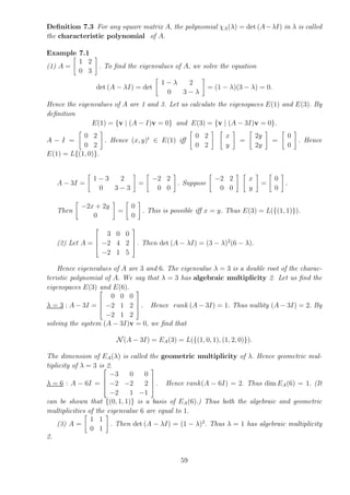
4. (−1)n
λn
+ (−1)n−1
λn−1
(a11 + . . . + ann) + . . . (48)
Put λ = 0 to get det A = constant term of det (A − λI).
Since λ1, λ2, . . . , λn are roots of det (A − λI) = 0 we have
det (A − λI) = (−1)n
(λ − λ1)(λ − λ2) . . . (λ − λn). (49)
(50)
(−1)n
[λn
− (λ1 + λ2 + . . . + λn)λn−1
+ . . . + (−1)n
λ1λ2 . . . λn]. (51)
Comparing (49) and 51), we get, the constant term of det (A − λI) is equal to λ1λ2 . . . λn =
det A and tr(A) = a11 + a22 + . . . + ann = λ1 + λ2 + . . . + λn. ♠
Proposition 7.3 Let v1, v2, . . . , vk be eigenvectors of a matrix A associated to distinct
eigenvalues λ1, λ2, . . . , λk. Then v1, v2, . . . , vk are linearly independent.
Proof: Apply induction on k. It is clear for k = 1. Suppose k ≥ 2 and c1v1 + . . . + ckvk = 0
for some scalars c1, c2, . . . , ck. Hence c1Av1 + c2Av2 + . . . + ckAvk = 0
Hence
c1λ1v1 + c2λ2v2 + . . . + ckλkvk = 0
Hence
λ1(c1v1 + c2v2 + . . . + ckvk) − (λ1c1v1 + λ2c2v2 + . . . + λkckvk)
= (λ1 − λ2)c2v2 + (λ1 − λ3)c3v3 + . . . + (λ1 − λk)ckvk = 0
By induction, v2, v3, . . ., vk are linearly independent. Hence (λ1 − λj)cj = 0 for j =
2, 3, . . ., k. Since λ1 6= λj for j = 2, 3, . . ., k, cj = 0 for j = 2, 3, . . ., k. Hence c1 is also
zero. Thus v1, v2, . . . , vk are linearly independent. ♠
Proposition 7.4 Suppose A is an n×n matrix. Let A have n distinct eigenvalues λ1, λ2, . . . , λn.
Let C be the matrix whose column vectors are respectively v1, v2, . . . , vn where vi is an eigen-
vector for λi for i = 1, 2, . . . , n. Then
C−1
AC = D(λ1, . . ., λn) = D
the diagonal matrix.
Proof: It is enough to prove AC = CD. For i = 1, 2, . . ., n : let Ci
(= vi) denote the ith
column of C etc.. Then
(AC)i
= ACi
= Avi = λivi.
Similarly,
(CD)i
= CDi
= λivi.
Hence AC = CD as required.] ♠
61

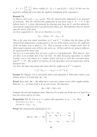
5. 7.3 Relation Between Algebraic and Geometric Multiplicities
Recall that
Definition 7.4 The algebraic multiplicity aA(µ) of an eigenvalue µ of a matrix A is defined
to be the multiplicity k of the root µ of the polynomial χA(λ). This means that (λ−µ)k
divides
χA(λ) whereas (λ − µ)k+1
does not.
Definition 7.5 The geometric multiplicity of an eigenvalue µ of A is defined to be the
dimension of the eigenspace EA(λ);
gA(λ) := dim EA(λ).
Proposition 7.5 Both algebraic multiplicity and the geometric multiplicities are invariant
of similarity.
Proof: We have already seen that for any invertible matrix C, χA(λ) = χC−1AC(λ). Thus
the invariance of algebraic multiplicity is clear. On the other hand check that EC−1AC(λ) =
C(EA(λ)). Therefore, dim (EC−1AC(λ)) = dim C(EAλ)) = dim (EA(λ)), the last equality
being the consequence of invertibility of C.
♠
We have observed in a few examples that the geometric multiplicity of an eigenvalue is
at most its algebraic multiplicity. This is true in general.
Proposition 7.6 Let A be an n×n matrix. Then the geometric multiplicity of an eigenvalue
µ of A is less than or equal to the algebraic multiplicity of µ.
Proof: Put aA(µ) = k. Then (λ − µ)k
divides det (A − λI) but (λ − µ)k+1
does not.
Let gA(µ) = g, be the geometric multiplicity of µ. Then EA(µ) has a basis consisting
of g eigenvectors v1, v2, . . . , vg. We can extend this basis of EA(µ) to a basis of Cn
, say
{v1, v2, . . . , vg, . . . , vn}. Let B be the matrix such that Bj
= vj. Then B is an invertible
matrix and
B−1
AB =






µIg X
0 Y






where X is a g × (n − g) matrix and Y is an (n − g) × (n − g) matrix. Therefore,
det (A − λI) = det [B−1
(A − λI)B] = det (B−1
AB − λI)
= (det (µ − λ)Ig)(det (C − λIn−g)
= (µ − λ)g
det (Y − λIn−g).
Thus g ≤ k. ♠
Remark 7.4 We will now be able to say something about the diagonalizability of a given
matrix A. Assuming that there exists B such that B−1
AB = D(λ1, . . . , λn), as seen in the
previous proposition, it follows that AB = BD . . . etc.. ABi
= λBi
where Bi
denotes the
ith
column vector of B. Thus we need not hunt for B anywhere but look for eigenvectors of
A. Of course Bi
are linearly independent, since B is invertible. Now the problem turns to
62

6. the question whether we have n linearly independent eigenvectors of A so that they can be
chosen for the columns of B. The previous proposition took care of one such case, viz., when
the eigenvalues are distinct. In general, this condition is not forced on us. Observe that the
geometric multiplicity and algebraic multiplicity of an eigenvalue co-incide for a diagonal
matrix. Since these concepts are similarity invariants, it is necessary that the same is true
for any matrix which is diagonalizable. This turns out to be sufficient also. The following
theorem gives the correct condition for diagonalization.
Theorem 7.1 A n × n matrix A is diagonalizable if and only if for each eigenvalue µ of A
we have the algebraic and geometric multiplicities are equal: aA(µ) = gA(µ).
Proof: We have already seen the necessity of the condition. To prove the converse, suppose
that the two multiplicities coincide for each eigenvalue. Suppose that λ1, λ2, . . . , λk are all
the eigenvalues of A with algebraic multiplicities n1, n2, . . ., nk. Let
B1 = {v11, v12, . . . , v1n1 } = a basis of E(λ1),
B2 = {v21, v22, . . . , v2n2 } = a basis of E(λ2),
.
.
.
Bk = {vk1, vk2, . . . , vknk
} = a basis of E(λk).
Use induction on k to show that B = B1 ∪ B2 ∪ . . . ∪ Bk is a linearly independent set. (The
proof is exactly similar to the proof of proposition (7.3). Denote the matrix with columns
as elements of the basis B also by B itself. Then, check that B−1
AB is a diagonal matrix.
Hence A is diagonalizable. ♠
63

7. Lectures 19,20,21
7.4 Eigenvalues of Special Matrices
In this section we discuss eigenvalues of special matrices. We will work in the n-dimensional
complex vector space Cn
. If u = (u1, u2, . . . , un)t
and v = (v1, v2, . . . , vn)t
∈ Cn
, we have
defined their inner product in Cn
by
hu, vi = u∗
v = u1v1 + u2v2 + · · · + unvn.
The length of u is given by kuk =
q
|u1|2 + · · · + |un|2.
Definition 7.6 Let A be a square matrix with complex entries. A is called
(i) Hermitian if A = A∗
;
(ii) Skew Hermitian if A = −A∗
.
Lemma 7.2 A is Hermitian iff for all column vectors v, w we have
(Av)∗
w = v∗
Aw; i.e., (hAv, wi = hv, Awi) (52)
Proof: If A is Hermitian then (Av)∗
w = v∗
A∗
w = v∗
Aw. To see the converse, take v, w to
be standard basic column vectors. ♠
Remark 7.5
(i) If A is real then A = A∗
means A = At
. Hence real symmetric matrices are Hermitian.
Likewise a real skew Hermitian matrix is skew symmetric.
(ii) A is Hermitian iff ıA is skew Hermitian.
Proposition 7.7 Let A be an n × n Hermitian matrix. Then :
1. For any u ∈ Cn
, u∗
Au is a real number.
2. All eigenvalues of A are real.
3. Eigenvectors of a Hermitian matrix corresponding to distinct eigenvalues are mutually
orthogonal.
Proof: (1) Since u∗
Au is a complex number, to prove it is real, we prove that (u∗
Au)∗
=
u∗
Au. But (u∗
Au)∗
= u∗
A∗
(u∗
)∗
= u∗
Au. Hence u∗
Au is real for all u ∈ Cn
.
(2) Suppose λ is an eigenvalue of A and u is an eigenvector for λ. Then
u∗
Au = u∗
(λu) = λ(u∗
u) = λkuk2
.
Since u∗
Au is real and kuk is a nonzero real number, it follows that λ is real.
(3) Let λ and µ be two distinct eigenvalues of A and u and v be corresponding eigenvec-
tors. Then Au = λu and Av = µv. Hence
λu∗
v = (λu)∗
v = (Au)∗
v = u∗
(Av) = u∗
µv = µ(u∗
v).
Hence (λ − µ)u∗
v = 0. Since λ 6= µ, u∗
v = 0. ♠
64

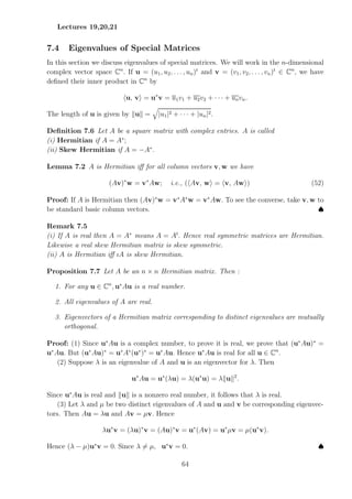
8. Corollary 7.1 Let A be an n × n skew Hermitian matrix. Then :
1. For any u ∈ Cn
, u∗
Au is either zero or a purely imaginary number.
2. Each eigenvalue of A is either zero or a purely imaginary number.
3. Eigenvectors of A corresponding to distinct eigenvalues are mutually orthogonal.
Proof: All this follow straight way from the corresponding statement about Hermitian
matrix, once we note that A is skew Hermitian implies ıA is Hermitian and the fact that a
complex number c is real iff ıc is either zero or purely imaginary.
Definition 7.7 Let A be a square matrix over C. A is called
(i) unitary if A∗
A = I;
(ii) orthogonal if A is real and unitary.
Thus a real matrix A is orthogonal iff AT
= A−1
. Also observe that A is unitary iff AT
is
unitary iff A is unitary.
Example 7.2 The matrices
U =
"
cos θ sin θ
− sin θ cos θ
#
and V =
1
√
2
"
1 i
i 1
#
are orthogonal and unitary respectively.
Proposition 7.8 Let A be a square matrix. Then the following conditions are equivalent.
(i) U is unitary.
(ii) The rows of U form an orthonormal set of vectors.
(iii) The columns of U form an orthonormal set of vectors.
(iv) U preserves the inner product, i.e., for all vectors x, y ∈ Cn
, we have hUx, Uyi = hx, yi.
Proof: Write the matrix U column-wise :
U = [u1 u2 . . . un] so that U∗
=







u∗
1
u∗
2
.
.
.
u∗
n







.
Hence
U∗
U =







u∗
1
u∗
2
.
.
.
u∗
n







[u1 u2 . . . un]
=







u∗
1u1 u∗
1u2 · · · u∗
1un
u∗
2u1 u∗
2u2 · · · u∗
2un
.
.
. · · ·
u∗
nu1 u∗
nu2 · · · u∗
nun







.
65

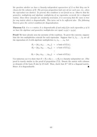
9. Thus U∗
U = I iff u∗
i uj = 0 for i 6= j and u∗
i ui = 1 for i = 1, 2, . . . , n iff the column vectors
of U form an orthonormal set. This proves (i) ⇐⇒ (ii). Since U∗
U = I implies UU∗
= I,
the proof of (i) ⇐⇒ (iii) follows.
To prove (i) ⇐⇒ (iv) let U be unitary. Then U∗
U = Id and hence hUx, Uyi = hx, U∗
Uyi =
hx, yi. Conversely, iff U preserves inner product take x = ei and y = ej to get
e∗
i (U∗
U)ej = e∗
i ej = δij
where δij are Kronecker symbols (δij = 1 if i = j; = 0 otherwise.) This means the (i, j)th
entry of U∗
U is δij. Hence U∗
U = In. ♠
Remark 7.6 Observe that the above theorem is valid for an orthogonal matrix also by merely
applying it for a real matrix.
Corollary 7.2 Let U be a unitary matrix. Then :
(1) For all x, y ∈ Cn
, hUx, Uyi = hx, yi. Hence kUxk = kxk.
(2) If λ is an eigenvalue of U then |λ| = 1.
(3) Eigenvectors corresponding to different eigenvalues are orthogonal.
Proof: (1) We have, kUxk2
= hUx, Uxi = hx, xi = kxk2
.
(2) If λ is an eigenvalue of U with eigenvector x then Ux = λx. Hence kxk = kUxk = |λ| kxk.
Hence |λ| = 1.
(3) Let Ux = λx and Uy = µy where x, y are eigenvectors with distinct eigenvalues λ and
µ respectively. Then
hx, yi = hUx, Uyi = hλx, µyi = λµhx, yi.
Hence λµ = 1 or hx, yi = 0. Since λλ = 1, we cannot have λµ = 1. Hence hx, yi = 0, i.e., x
and y are orthogonal. ♠
Example 7.3 U =
"
cos θ − sin θ
sin θ cos θ
#
is an orthogonal matrix. The characteristic polyno-
mial of U is :
D(λ) = det (U − λI) = det,
"
cos θ − λ − sin θ
sin θ cos θ − λ
#
= λ2
− 2λ cos θ + 1.
Roots of D(λ) = 0 are :
λ =
2 cos θ ±
√
4cos2θ − 4
2
= cos θ ± ı sin θ = e±ıθ
.
Hence |λ| = 1. Check that eigenvectors are :
for λ = eıθ
: x =
"
1
−ı
#
and for λ = e−ıθ
: y =
"
1
ı
#
.
Thus x∗
y = [1 ı]
"
1
ı
#
= 1 + ı2
= 0. Hence x ⊥ y. Normalize the eigenvectors x and y.
Therefore if we take,
C =
1
√
2
"
1 1
−ı ı
#
then C−1
UC = D(eıθ
, e−ıθ
).
66