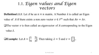
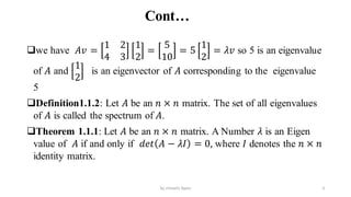
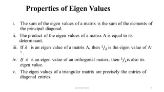
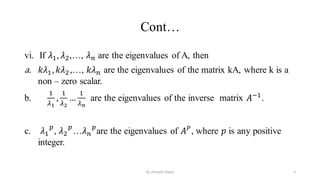
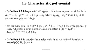
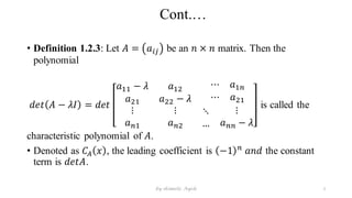
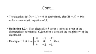
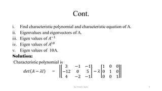
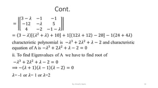
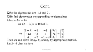
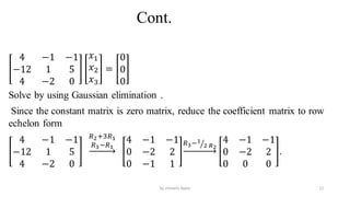
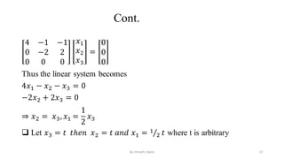
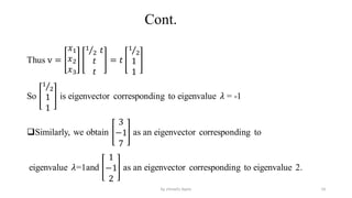
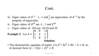
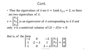
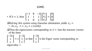
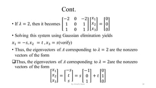
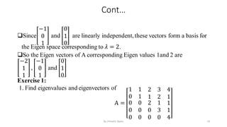
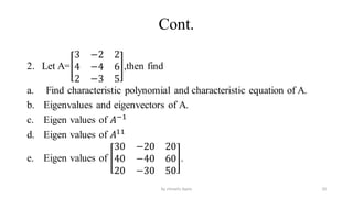
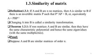
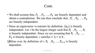
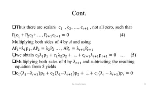
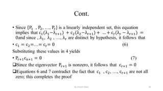
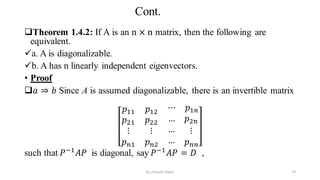
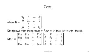
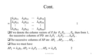
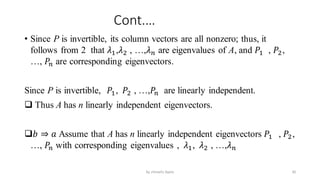
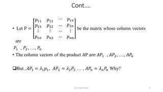
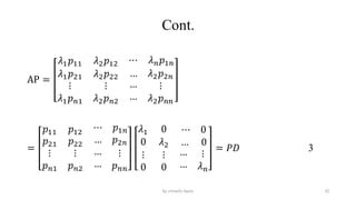
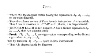
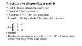
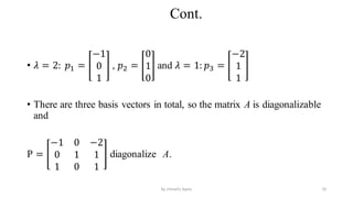
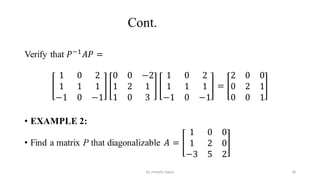
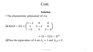
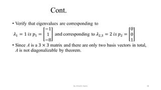
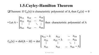
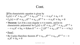
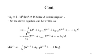
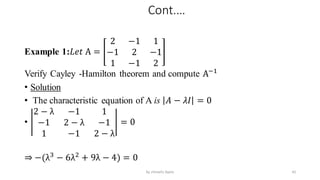
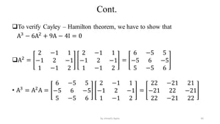
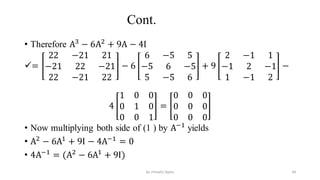
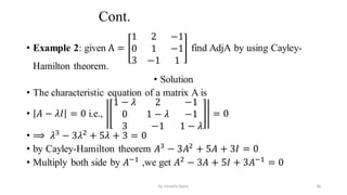
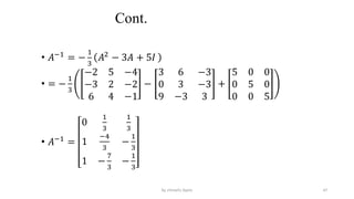
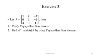
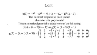
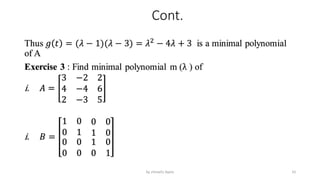
The document discusses eigenvalues and eigenvectors as essential concepts in linear algebra, detailing their definitions, properties, and the calculation of characteristic polynomials and equations for matrices. It also introduces the concepts of matrix similarity and diagonalization, highlighting the criteria for a matrix to be diagonalizable and the implications of having linearly independent eigenvectors. Several examples and exercises are provided to illustrate these concepts and reinforce understanding.

1. LINEAR ALGEBRA II
Chapter one
Characteristic Equation
1
by shimelis Ayele

2. 1.1. Eigen values and Eigen
vectors
2
by shimelis Ayele

3. Cont…
we have 𝐴𝑣 =
1 2
4 3
1
2
=
5
10
= 5
1
2
= 𝜆𝑣 so 5 is an eigenvalue
of 𝐴 and
1
2
is an eigenvector of 𝐴 corresponding to the eigenvalue
5
Definition1.1.2: Let 𝐴 be an 𝑛 × 𝑛 matrix. The set of all eigenvalues
of 𝐴 is called the spectrum of 𝐴.
Theorem 1.1.1: Let 𝐴 be an 𝑛 × 𝑛 matrix. A Number 𝜆 is an Eigen
value of 𝐴 if and only if 𝑑𝑒𝑡 𝐴 − 𝜆𝐼 = 0, where 𝐼 denotes the 𝑛 × 𝑛
identity matrix.
3
by shimelis Ayele

4. Properties of Eigen Values
i. The sum of the eigen values of a matrix is the sum of the elements of
the principal diagonal.
ii. The product of the eigen values of a matrix A is equal to its
determinant.
iii. If 𝜆 is an eigen value of a matrix A, then Τ
1
𝜆 is the eigen value of A-
1 .
iv. If 𝜆 is an eigen value of an orthogonal matrix, then Τ
1
𝜆is also its
eigen value.
v. The eigen values of a triangular matrix are precisely the entries of
diagonal entries.
4
by shimelis Ayele

5. Cont…
vi. If 𝜆1, 𝜆2,…, 𝜆𝑛 are the eigenvalues of A, then
a. 𝑘𝜆1,𝑘𝜆2,…, 𝑘𝜆𝑛 are the eigenvalues of the matrix kA, where k is a
non – zero scalar.
b.
1
𝜆1
,
1
𝜆2
…
1
𝜆𝑛
are the eigenvalues of the inverse matrix 𝐴−1
.
c. 𝜆1
𝑝
, 𝜆2
𝑝
…𝜆𝑛
𝑝
are the eigenvalues of 𝐴𝑃
, where 𝑝 is any positive
integer.
5
by shimelis Ayele

6. 1.2 Characteristic polynomial
• Definition 1.2.1:Polynomial of degree 𝑛 in 𝑥 is an expression of the form
𝑎𝑛𝑥𝑛
+ 𝑎𝑛−1𝑥𝑛−1
+ ⋯ + 𝑎1𝑥 + 𝑎0, where 𝑎0,𝑎1,…𝑎𝑛 ∈ 𝐹 𝑎𝑛𝑑 𝑎𝑛 ≠ 0
, 𝑛 𝑖𝑠 𝑛𝑜𝑛 𝑛𝑒𝑔𝑎𝑡𝑖𝑣𝑒 𝑖𝑛𝑡𝑒𝑔𝑒𝑟.
• We can write 𝑝 𝑥 = 𝑎𝑛𝑥𝑛
+ 𝑎𝑛−1𝑥𝑛−1
+ ⋯ + 𝑎1𝑥 + 𝑎0, if we replace x
every where by a given number 𝜆 and we obtain 𝑝 𝜆 = 𝑎𝑛𝜆𝑛
+
𝑎𝑛−1𝜆𝑛−1
+ ⋯ + 𝑎1𝜆 + 𝑎0
• Definition 1.2.2: Let 𝑝 𝑥 be a polynomial in x. A number 𝜆 is called a
root of 𝑝 𝑥 if 𝑝 𝜆 = 0.
6
by shimelis Ayele

7. Cont.…
• Definition 1.2.3: Let 𝐴 = 𝑎𝑖𝑗 be an 𝑛 × 𝑛 matrix. Then the
polynomial
𝑑𝑒𝑡 𝐴 − 𝜆𝐼 = 𝑑𝑒𝑡
𝑎11 − 𝜆 𝑎12
⋯ 𝑎1𝑛
𝑎21 𝑎22 − 𝜆 ⋯ 𝑎21
⋮
𝑎𝑛1
⋮
𝑎𝑛2
⋱
…
⋮
𝑎𝑛𝑛 − 𝜆
is called the
characteristic polynomial of 𝐴.
• Denoted as 𝐶𝐴 𝑥 , the leading coefficient is −1 𝑛
𝑎𝑛𝑑 the constant
term is 𝑑𝑒𝑡𝐴.
7
by shimelis Ayele

8. Cont…
• The equation 𝑑𝑒𝑡 𝐴 − 𝜆𝐼 = 0 or equivalently 𝑑𝑒𝑡 𝜆𝐼 − 𝐴 = 0 is
called characteristic equation of 𝐴.
• Definition 1.2.4: If an eigenvalue 𝜆 occur k times as a root of the
characteristic polynomial 𝐶𝐴 𝑥 , then k is called the multiplicity of the
eigenvalue .
• Example 1: Let 𝐴 =
3 −1 −1
−12 0 5
4 −2 −1
then,
8
by shimelis Ayele

9. Cont.
i. Find characteristic polynomial and characteristic equation of A.
ii. Eigenvalues and eigenvectors of A.
iii. Eigen values of 𝐴−1
iv. Eigen values of 𝐴10
v. Eigen values of 10A.
Solution:
Characteristic polynomial is
𝑑𝑒𝑡 𝐴 − 𝜆𝐼 =
3 −1 −1
−12 0 5
4 −2 −1
− 𝜆
1 0 0
0 1 0
0 0 1
9
by shimelis Ayele

10. Cont.
=
3 − 𝜆 −1 −1
−12 −𝜆 5
4 −2 −1 − 𝜆
= 3 − 𝜆 𝜆2
+ 𝜆 + 10 + 1 12𝜆 + 12 − 20 − 1 24 + 4𝜆
characteristic polynomial is −𝜆3
+ 2𝜆2
+ 𝜆 − 2 and characteristic
equation of A is −𝜆3
+ 2𝜆2
+ 𝜆 − 2 = 0
ii. To find Eigenvalues of A we have to find root of
−𝜆3
+ 2𝜆2
+ 𝜆 − 2 = 0
⟹ − 𝜆 + 1 𝜆 − 1 𝜆 − 2 = 0
𝜆= -1 or 𝜆= 1 or 𝜆=2
10
by shimelis Ayele

11. Cont.
So the eigenvalues are -1,1 and 2 .
To find eigenvector corresponding to eigenvalues
write 𝐴𝑣 = 𝜆𝑣
⟹ 𝐴 − 𝜆𝐼 𝑣 = 0 that is
⟹
3 − 𝜆 −1 −1
−12 −𝜆 5
4 −2 −1 − 𝜆
𝑥1
𝑥2
𝑥3
=
0
0
0
Then we can solve for 𝑥1, 𝑥2 and 𝑥3 by appropriate method.
Let 𝜆= -1 ,then we have
11
by shimelis Ayele

12. Cont.
4 −1 −1
−12 1 5
4 −2 0
𝑥1
𝑥2
𝑥3
=
0
0
0
Solve by using Gaussian elimination .
Since the constant matrix is zero matrix, reduce the coefficient matrix to row
echelon form
4 −1 −1
−12 1 5
4 −2 0
𝑅2+3𝑅1
𝑅3−𝑅1
4 −1 −1
0 −2 2
0 −1 1
𝑅3− ൗ
1
2 𝑅2
4 −1 −1
0 −2 2
0 0 0
.
12
by shimelis Ayele

13. Cont.
4 −1 −1
0 −2 2
0 0 0
𝑥1
𝑥2
𝑥3
=
0
0
0
Thus the linear system becomes
4𝑥1 − 𝑥2 − 𝑥3 = 0
−2𝑥2 + 2𝑥3 = 0
⇒ 𝑥2 = 𝑥3,𝑥1 =
1
2
𝑥3
 Let 𝑥3 = 𝑡 𝑡ℎ𝑒𝑛 𝑥2 = 𝑡 𝑎𝑛𝑑 𝑥1 = Τ
1
2 𝑡 where t is arbitrary
13
by shimelis Ayele

14. Cont.
Thus v =
𝑥1
𝑥2
𝑥3
Τ
1
2 𝑡
𝑡
𝑡
= 𝑡
Τ
1
2
1
1
So
Τ
1
2
1
1
is eigenvector corresponding to eigenvalue 𝜆 = -1
Similarly, we obtain
3
−1
7
as an eigenvector corresponding to
eigenvalue 𝜆=1and
1
−1
2
as an eigenvector corresponding to eigenvalue 2.
14
by shimelis Ayele

15. Cont.
iii. Eigen values of 𝐴−1
. 1, -1 and
1
2
are eigenvalues of 𝐴−1
by the
property of eigenvalue.
iv. Eigen values of 𝐴10
are -1 , 1 and 210
v. Eigen values of 10A are -10,10 and 20
Example 2: Let 𝐴 =
0 0 −2
1 2 1
1 0 3
Solution:
• The characteristic equation of matrix A is 𝜆3
−5𝜆2
+ 8𝜆 − 4 = 0, or,
in factored form 𝜆 − 1 𝜆 − 2 2
= 0
15
by shimelis Ayele

16. Cont.
• Thus the eigenvalues of A are 𝜆 = 1and 𝜆2,3 = 2, so there
are two eigenvalues of A.
v =
𝑥1
𝑥2
𝑥3
,is an eigenvector of A corresponding to 𝜆 if and
only v is a nontrivial solution of 𝐴 − 𝜆𝐼 𝑣 = 0
that is, of the form
−𝜆 0 −2
1 2 − 𝜆 1
1 0 3 − 𝜆
𝑥1
𝑥2
𝑥3
=
0
0
0
16
by shimelis Ayele

17. cont.
• If 𝜆 = 1, then
−1 0 −2
1 1 1
1 0 2
𝑥1
𝑥2
𝑥3
=
0
0
0
Solving this system using Gaussian elimination yields 𝑥1 =
− 2𝑠, 𝑥2 = 𝑠 , 𝑥3 = 𝑠 (verify)
Thus the eigenvectors corresponding to 𝜆 = 1are the nonzero vectors
of the form
−2𝑠
𝑠
𝑠
= 𝑠
−2
1
1
so that
−2
1
1
is the Eigen vector corresponding to
eigenvalue 1
17
by shimelis Ayele

18. Cont.
• If 𝜆 = 2, then it becomes
−2 0 −2
1 0 1
1 0 1
𝑥1
𝑥2
𝑥3
=
0
0
0
• Solving this system using Gaussian elimination yields
𝑥1 = −𝑠, 𝑥2 = 𝑡 , 𝑥3 = 𝑠(verify)
• Thus, the eigenvectors of A corresponding to 𝜆 = 2 are the nonzero
vectors of the form
Thus, the eigenvectors of A corresponding to 𝜆 = 2are the nonzero
vectors of the form
𝑥1
𝑥2
𝑥3
=
−𝑠
𝑡
𝑠
= 𝑠
−1
0
1
+ 𝑡
0
1
0 18
by shimelis Ayele

19. Cont…
Since
−1
0
1
and
0
1
0
are linearly independent,these vectors form a basis for
the Eigen space corresponding to 𝜆 = 2.
So the Eigen vectors of A corresponding Eigen values 1and 2 are
−2
1
1
,
−1
0
1
and
0
1
0
Exercise 1:
1. Find eigenvalues and eigenvectors of
A =
1 1 2 3 4
0 1 1 2 1
0
0
0
0
0
0
2
0
0
1
3
0
1
1
4 19
by shimelis Ayele

20. Cont.
2. Let A=
3 −2 2
4 −4 6
2 −3 5
,then find
a. Find characteristic polynomial and characteristic equation of A.
b. Eigenvalues and eigenvectors of A.
c. Eigen values of 𝐴−1
d. Eigen values of 𝐴11
e. Eigen values of
30 −20 20
40 −40 60
20 −30 50
.
20
by shimelis Ayele

21. 1.3.Similarity of matrix
Definition1.3.1: If A and B are n xn matrices, then A is similar to B if
there is an invertible matrix P such that P-1AP = B, or, equivalently
A = PBP-1
Changing A into B is called a similarity transformation.
Theorem 1.3.1: If nxn matrices A and B are similar, then they have
the same characteristic polynomial and hence the same eigenvalues
(with the same multiplicities).
Proof:
Suppose A and B are similar matrices of order n.
21
by shimelis Ayele

22. Cont.
The characteristic polynomial of B is given by
det B − λI
= det P−1AP − λI
= det p−1
𝐴 − λI p
= det(p−1
)det A − λI det(p )
= det(p−1
p) det A − λI
= det A − λI
Definition 1.3.2: The set of distinct eigenvalues, denoted by σ(A) , is
called the spectrum of A.
Definition 1.3.3:For square matrices A , the number ρ(A) =
max 𝜆 , λ∈ σ(A)is called the spectral radius of A.
22
by shimelis Ayele

23. 1.4. Diagonalization
• Definition1.4.1: A square matrix A is called diagonalizable if there
exist an invertible matrix P such that 𝑃−1
𝐴𝑃 is a diagonal matrix; the
matrix P is said to diagonalize A.
THEOREM 1.4.1 : If 𝑃1 , 𝑃2, …, 𝑃𝑘 are Eigen vectors of A
corresponding to distinct eigenvalues
,λ1, λ2 , …,λk then {P1 , P2, …, Pk } is a linearly independent set.
• Proof
 Let , 𝑃1 , 𝑃2, …, 𝑃𝑘 be eigenvectors of A corresponding to distinct
eigenvalues 𝜆1, 𝜆2 , …,𝜆𝑘 .
23
by shimelis Ayele

24. Cont.
• We shall assume that, 𝑃1 , 𝑃2, …, 𝑃𝑘 are linearly dependent and
obtain a contradiction. We can then conclude that , P1 , P2, …, Pk
are linearly independent.
• Since an eigenvector is nonzero by definition, p1 is linearly
independent. Let r be the largest integer such that P1 , P2, …, Pr
is linearly independent. Since we are assuming that P1 , P2, …,
Pk is linearly dependent, r satisfies 1 ≤ r ≤ k .
More over, by definition of r, P1 , P2, …, Pr+1 is linearly
dependent.
24
by shimelis Ayele

25. Cont.
Thus there are scalars c1 , c2, …, cr+1 , not all zero, such that
P1c1 + P2c2+ …, Pr+1cr+1 = 0 (4)
Multiplying both sides of 4 by A and using
AP1=λ1p1, AP2 = λ2P2 … , APn = λr+1Pr+1
we obtain c1λ1p1 + c2λ2p2 + … + cr+1λr+1pr+1 = 0 … (5)
Multiplying both sides of 4 by λr+1 and subtracting the resulting
equation from 5 yields
c1(λ1−λr+1)p1 + c2(λ2−λr+1)p2 + … + cr(λr − λr+1)pr = 0
25
by shimelis Ayele

26. Cont.
• Since P1 , P2, …, Pr is a linearly independent set, this equation
implies that c1(λ1−λr+1) + c2(λ2−λr+1) + … + cr(λr − λr+1) =
0and since , λ1, λ2 , …, λr are distinct by hypothesis, it follows that
• c1 = c2=…= cr= 0 (6)
Substituting these values in 4 yields
• Pr+1cn+1 = 0 (7)
Since the eigenvector Pr+1 is nonzero, it follows that cr+1 = 0
Equations 6 and 7 contradict the fact that c1 , c2, …, cr+1 are not all
zero; this completes the proof
26
by shimelis Ayele

27. Cont.
Theorem 1.4.2: If A is an n × n matrix, then the following are
equivalent.
a. A is diagonalizable.
b. A has n linearly independent eigenvectors.
• Proof
𝑎 ⇒ 𝑏 Since A is assumed diagonalizable, there is an invertible matrix
𝑝11 𝑝12
⋯ 𝑝1𝑛
𝑝21 𝑝22 … 𝑝2𝑛
⋮
𝑝𝑛1
⋮
𝑝𝑛2
…
…
⋮
𝑝𝑛𝑛
such that 𝑃−1
𝐴𝑃 is diagonal, say 𝑃−1
𝐴𝑃 = 𝐷 ,
27
by shimelis Ayele

28. Cont.
where D =
𝜆1 0 ⋯ 0
0 𝜆2 … 0
⋮
0
⋮
0
…
…
⋮
𝜆𝑛
It follows from the formula 𝑃−1
𝐴𝑃 = 𝐷 that 𝐴𝑃 = 𝑃𝐷 ; that is ,
AP =
𝑝11 𝑝12
⋯ 𝑝1𝑛
𝑝21 𝑝22 … 𝑝2𝑛
⋮
𝑝𝑛1
⋮
𝑝𝑛2
…
…
⋮
𝑝𝑛𝑛
𝜆1 0 ⋯ 0
0 𝜆2 … 0
⋮
0
⋮
0
…
…
⋮
𝜆𝑛
28
by shimelis Ayele

29. Cont.
=
𝜆1𝑝11 𝜆2𝑝12 ⋯ 𝜆𝑛𝑝1𝑛
𝜆1𝑝21 𝜆2𝑝22 … 𝜆𝑛𝑝2𝑛
⋮
𝜆1𝑝𝑛1
⋮
𝜆2𝑝𝑛2
…
…
⋮
𝜆𝑛𝑝𝑛𝑛
1
If we denote the column vectors of P,𝑏𝑦 𝑃1,𝑃2, …, 𝑃𝑛, then from 1,
the successive columns of PD are 𝜆1𝑃1 , 𝜆2𝑃2, …, 𝜆𝑛𝑃𝑛 .
The successive columns of AP are 𝐴𝑃1 , 𝐴𝑃2, …, 𝐴𝑃𝑛 .
Thus we must have
𝐴𝑃1 = 𝜆1𝑝1, 𝐴𝑃2 = 𝜆2𝑃2 … , 𝐴𝑃𝑛 = 𝜆𝑛𝑃𝑛 2
29
by shimelis Ayele

30. Cont.…
• Since P is invertible, its column vectors are all nonzero; thus, it
follows from 2 that 𝜆1,𝜆2 , …,𝜆𝑛 are eigenvalues of A, and 𝑃1 , 𝑃2,
…, 𝑃𝑛 are corresponding eigenvectors.
Since P is invertible, 𝑃1, 𝑃2 , …,𝑃𝑛 are linearly independent.
 Thus A has n linearly independent eigenvectors.
𝑏 ⇒ 𝑎 Assume that A has n linearly independent eigenvectors 𝑃1 , 𝑃2,
…, 𝑃𝑛 with corresponding eigenvalues , 𝜆1, 𝜆2 , …,𝜆𝑛
30
by shimelis Ayele

31. Cont.…
• Let P =
𝑝11 𝑝12
⋯ 𝑝1𝑛
𝑝21 𝑝22 … 𝑝2𝑛
⋮
𝑝𝑛1
⋮
𝑝𝑛2
…
…
⋮
𝑝𝑛𝑛
be the matrix whose column vectors
are
𝑃1 , 𝑃2, …, 𝑃𝑛
• The column vectors of the product AP are 𝐴𝑃1 , 𝐴𝑃2, …, 𝐴𝑃𝑛
But ,𝐴𝑃1 = 𝜆1𝑝1, 𝐴𝑃2 = 𝜆2𝑃2 … , 𝐴𝑃𝑛 = 𝜆𝑛𝑃𝑛 Why?
31
by shimelis Ayele

32. Cont.
AP =
𝜆1𝑝11 𝜆2𝑝12 ⋯ 𝜆𝑛𝑝1𝑛
𝜆1𝑝21 𝜆2𝑝22 … 𝜆2𝑝2𝑛
⋮
𝜆1𝑝𝑛1
⋮
𝜆2𝑝𝑛2
…
…
⋮
𝜆2𝑝𝑛𝑛
=
𝑝11 𝑝12
⋯ 𝑝1𝑛
𝑝21 𝑝22 … 𝑝2𝑛
⋮
𝑝𝑛1
⋮
𝑝𝑛2
…
…
⋮
𝑝𝑛𝑛
𝜆1 0 ⋯ 0
0 𝜆2 … 0
⋮
0
⋮
0
…
…
⋮
𝜆𝑛
= 𝑃𝐷 3
32
by shimelis Ayele

33. Cont.
• Where D is the diagonal matrix having the eigenvalues, 𝜆1, 𝜆2 , …,𝜆𝑛
on the main diagonal.
• Since the column vectors of P are linearly independent, P is invertible.
Thus 3 can be rewritten as 𝑃−1
𝐴𝑃 = 𝐷 ; that is, A is diagonalizable
• THEOREM 1.4.3: If an n × n matrix A has n distinct eigenvalues,λ1,
λ2 , …,λn then A is diagonalizable
• Proof: If P1 , P2, …, Pn are eigenvectors corresponding to the distinct
eigenvalues ,λ1, λ2 , …,λn
then by Theorem , P1 , P2, …, Pnare linearly independent.
• Thus A is diagonalizable by Theorem .
33
by shimelis Ayele

34. Procedure to diagonalize a matrix
 Find the linearly independent eigenvectors
 Construct P from eigenvectors
 Construct 𝐷 = 𝑃−1
𝐴𝑃 from eigenvalues
• Example 1: Finding a Matrix P that diagonalize a matrix A
A =
0 0 −2
1 2 1
1 0 3
• Solution
• The characteristic equation of A is 𝜆 − 1 𝜆 − 2 2
= 0 and we found
the following bases for the Eigen spaces:
34
by shimelis Ayele

35. Cont.
• 𝜆 = 2: 𝑝1 =
−1
0
1
, 𝑝2 =
0
1
0
and 𝜆 = 1: 𝑝3 =
−2
1
1
• There are three basis vectors in total, so the matrix A is diagonalizable
and
P =
−1 0 −2
0 1 1
1 0 1
diagonalize A.
35
by shimelis Ayele

36. Cont.
Verify that 𝑃−1
𝐴𝑃 =
1 0 2
1 1 1
−1 0 −1
0 0 −2
1 2 1
1 0 3
1 0 2
1 1 1
−1 0 −1
=
2 0 0
0 2 1
0 0 1
• EXAMPLE 2:
• Find a matrix P that diagonalizable 𝐴 =
1 0 0
1 2 0
−3 5 2
36
by shimelis Ayele

37. Cont.
Solution
• The characteristic polynomial of A is
 det 𝐴 − 𝜆𝐼 =
1 − 𝜆 0 0
1 2 − 𝜆 0
−3 5 2 − 𝜆
= 𝜆 − 1 𝜆 − 2 2
Thus the eigenvalues of A are 𝜆1 = 1 and 𝜆2,3= 2 .
37
by shimelis Ayele

38. Cont.
• Verify that eigenvalues are corresponding to
𝜆1 = 1 𝑖𝑠 𝑝1 =
−1
1
−8
and corresponding to 𝜆2,3 = 2 𝑖𝑠 𝑝2 =
0
0
1
• Since A is a 3 × 3 matrix and there are only two basis vectors in total,
A is not diagonalizable by theorem.
38
by shimelis Ayele

39. 1.5.Cayley-Hamilton Theorem
Theorem: If CA x is characteristic polynomial of A, then CA x = 0
• Let A =
a11 a12
… a1n
a21 a22
… a2n
⋮
an1
⋮
an2
⋱ ⋮
… ann
then characteristic polynomial of A
CA x = det A − λI = det
a11 − λ a12 … a1n
a21 a22 − λ … a2n
⋮
an1
⋮
an2
⋱ ⋮
… ann − λ
39
by shimelis Ayele

40. Cont.
The characteristic equation is given by
CA x = xn
+ an−1xn−1
+ an−2xn−2
+ ⋯ + a1x1
+ a0 = 0
• CA x = An
+ an−1An−1
+ an−2An−2
+ ⋯ + a1A1
+ Ia0 = 0
• Theorem: Let A be a non singular n × n matrix, and let its
characteristic polynomial be CA x = An
+ an−1An−1
+ an−2An−2
+
⋯ + a1A1
+ Ia0 = 0,then A−1
= −
1
a0
(An−1
+ an−1An−2
+ ⋯ + Ia1)
• Proof :
• By Cayley-Hamilton theorem An
+ an−1An−1
+ an−2An−2
+ ⋯ +
a1A1
+ Ia0 = 0
40
by shimelis Ayele

41. Cont.
• a0 = −1 n
detA ≠ 0, Since A is non singular .
• So the above equation can be written as
I = −
1
a0
(An
+ an−1An−1
+ an−2An−2
+ ⋯ + a1A1
= −
1
a0
(An−1
+ an−1An−2
+ ⋯ + Ia1)A
A−1
= −
1
a0
(An−1
+ an−1An−2
+ ⋯ + Ia1)
41
by shimelis Ayele

42. Cont.…
Example 1:𝐿𝑒𝑡 A =
2 −1 1
−1 2 −1
1 −1 2
Verify Cayley -Hamilton theorem and compute A−1
• Solution
• The characteristic equation of A is 𝐴 − 𝜆𝐼 = 0
•
2 − λ −1 1
−1 2 − λ −1
1 −1 2 − λ
= 0
⇒ −(λ3
− 6λ2
+ 9λ − 4) = 0
42
by shimelis Ayele

43. Cont.
To verify Cayley – Hamilton theorem, we have to show that
A3
− 6A2
+ 9A − 4I = 0
A2
=
2 −1 1
−1 2 −1
1 −1 2
2 −1 1
−1 2 −1
1 −1 2
=
6 −5 5
−5 6 −5
5 −5 6
• A3
= A2
A =
6 −5 5
−5 6 −5
5 −5 6
2 −1 1
−1 2 −1
1 −1 2
=
22 −21 21
−21 22 −21
22 −21 22
43
by shimelis Ayele

44. Cont.
• Therefore A3
− 6A2
+ 9A − 4I
=
22 −21 21
−21 22 −21
22 −21 22
− 6
6 −5 5
−5 6 −5
5 −5 6
+ 9
2 −1 1
−1 2 −1
1 −1 2
−
4
1 0 0
0 1 0
0 0 1
=
0 0 0
0 0 0
0 0 0
• Now multiplying both side of (1 ) by A−1
yields
• A2
− 6A1
+ 9I − 4A−1
= 0
• 4A−1
= (A2
− 6A1
+ 9I)
44
by shimelis Ayele

45. Cont.
4𝐴−1
=
6 −5 5
−5 6 −5
5 −5 6
− 6
2 −1 1
−1 2 −1
1 −1 2
+ 9
1 0 0
0 1 0
0 0 1
=
3 1 −1
1 3 1
−1 1 3
⟹ 𝐴−1
=
1
4
3 1 −1
1 3 1
−1 1 3
45
by shimelis Ayele

46. Cont.
• Example 2: given A =
1 2 −1
0 1 −1
3 −1 1
find AdjA by using Cayley-
Hamilton theorem.
• Solution
• The characteristic equation of a matrix A is
• 𝐴 − 𝜆𝐼 = 0 i.e.,
1 − 𝜆 2 −1
0 1 − 𝜆 −1
3 −1 1 − 𝜆
= 0
• ⟹ 𝜆3
− 3𝜆2
+ 5𝜆 + 3 = 0
• by Cayley-Hamilton theorem 𝐴3
− 3𝐴2
+ 5𝐴 + 3𝐼 = 0
• Multiply both side by 𝐴−1
,we get 𝐴2
− 3𝐴 + 5𝐼 + 3𝐴−1
= 0
46
by shimelis Ayele

47. Cont.
• 𝐴−1
= −
1
3
𝐴2
− 3𝐴 + 5𝐼
• = −
1
3
−2 5 −4
−3 2 −2
6 4 −1
−
3 6 −3
0 3 −3
9 −3 3
+
5 0 0
0 5 0
0 0 5
• 𝐴−1
=
0
1
3
1
3
1
−4
3
−
1
3
1 −
7
3
−
1
3
47
by shimelis Ayele

48. Cont.
• We know that , 𝐴−1
=
𝑎𝑑𝑗𝐴
𝐴
• Therefore 𝑎𝑑𝑗𝐴 = 𝐴 𝐴−1
= −3
0
1
3
1
3
1
−4
3
−
1
3
1 −
7
3
−
1
3
=
0 −1 −1
1 4 1
1 7 1
48
by shimelis Ayele

49. Cont.
• Another application of Cayley-Hamilton theorem is to compute power
of square matrix 𝐴
• Example: Let A =
2 5
1 −2
and then find A735
• Solution
• The characteristic polynomial of A is x2
− 9. Eigen values are -3,3 .
• Division algorithm applied to the polynomial x735
, x2
− 9 will give
equation of the form x735
= (x2
− 9)q x + a0 + a1x , (1)
Where a0 + a1x is remainder obtained by dividing x735
by x2
− 9.
49
by shimelis Ayele

50. Cont.
• Note that the degree of remainder is less than the degree of the
divisor x2
− 9.
• By Cayley-Hamilton theorem A2
− 9I = 0 .
• Inserting A for x in equation (1), we get
• A735
= a0 + a1A (2)
• Inserting eigen values 3 and -3 for x successively in equation (1), we
get
• 3735
= a0 + 3a1
50
by shimelis Ayele

51. Cont.…
• −3 735
= a0 − 3a1
• This gives a0 = 0, a1 = 3734
.
• Then A735
= a0 + a1A
• gives
• A735
= 3735
A.
51
by shimelis Ayele

52. 1.6.Minimal polynomial
• Definition 1.6.1: The minimal polynomial of a matrix A, denoted by 𝑚𝐴 𝜆
is the unique monic polynomial of least degree such that 𝑚𝐴 𝜆 = 0 .
• Theorem: a scalar 𝜆 is Eigen values of a matrix A if and only if is root of
minimal polynomial.
• proof(exercise)
• Example: find minimal polynomial 𝑚𝐴 𝜆 of 𝐴 =
2 2 −5
3 7 −15
1 2 −4
• Solution
• First find the characteristic polynomial of A.
52
by shimelis Ayele

53. Exercise 3
• Let 𝐴 =
1 2 −1
0 1 −1
3 −1 1
, then
1. Verify Cayley-Hamilton theorem
2. Find 𝐴−1
and AdjA by using Cayley-Hamilton theorem.
53
by shimelis Ayele

54. Cont.
•
p λ = −λ3
+ 5λ2
− 7λ + 3 = − λ − 1 2
λ − 3 .
The minimal polynomial must divid𝑒
characteristic polynomial.
Thus minimal polynomial is exactly one of the following
p λ = λ − 3 λ − 1 2
or g λ = λ − 3 λ − 1
g A = A − I A − 3I =
1 2 −5
3 6 −15
1 2 −5
−1 2 −5
3 4 −15
1 2 −7
=
0 0 0
0 0 0
0 0 0
54
by shimelis Ayele

55. Cont.
Thus 𝑔 𝑡 = (𝜆 − 1)(𝜆 − 3) = 𝜆2
− 4𝜆 + 3 is a minimal polynomial
of A
Exercise 3 : Find minimal polynomial m (λ ) of
i. 𝐴 =
3 −2 2
4 −4 6
2 −3 5
i. 𝐵 =
1 0 0 0
0 1 1 0
0
0
0
0
1 0
0 1
55
by shimelis Ayele