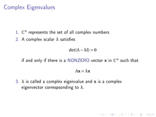
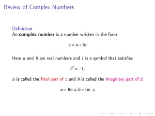
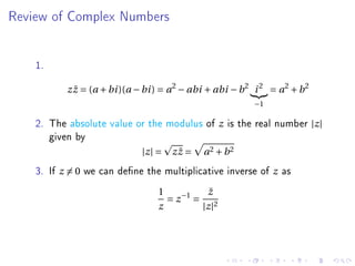
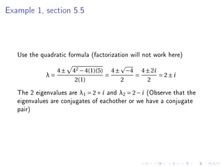
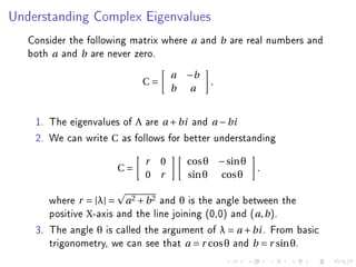
1. A complex number λ is an eigenvalue of a matrix A if there exists a non-zero vector x such that Ax = λx. 2. If a matrix has complex eigenvalues, it provides important information about the matrix, such as in problems involving vibrations and rotations in space. 3. For a complex eigenvalue λ = a + bi, a is called the real part and b is called the imaginary part. The absolute value |λ| represents the "length" or magnitude of the eigenvalue.

1. Announcements
Today's material will not be a part of Test 2.
Review for Test 2 tomorrow. Please come prepared with
questions.
Exam 2 will be on Feb 25 Thurs in class.
Please collect your graded exams on friday from Fisher 214.

2. Review of Complex Numbers
Denition
An complex number is a number written in the form
z = a + bi
Here a and b are real numbers and i is a symbol that satises
i 2 = −1.
a is called the Real part of z and b is called the Imaginary part of Z
a = Re z, b = Im z

3. Review of Complex Numbers
1. If 2 complex numbers are equal, their real and imaginary parts
must be the same.
2. Any real number a is a special complex number (a + 0i ).
3. You can add 2 complex numbers as
(a + bi ) + (c + d i ) = (a + c) + (b + d )i
You can multiply two complex numbers as
(a + bi )(c + d i ) = ac + ad i + bci + bd i 2 = (ac − bd ) + (ad + bc)i
−bd

4. Review of Complex Numbers
Denition
If z = a + bi is a complex number, we dene the conjugate of z
(denoted by z , read as z bar) as
¯
¯
z = a − bi
That is, we change the sign of the imaginary part of z .

5. Review of Complex Numbers
1.
z z = (a + bi )(a − bi ) = a 2 − abi + abi − b 2 i 2 = a 2 + b 2
¯
−1
2. The absolute value or the modulus of z is the real number |z|
given by
|z| = ¯
zz = a2 + b2
3. If z =0 we can dene the multiplicative inverse of z as
1 z¯
= z −1 = 2
z |z|

6. Back to Eigenvalues
1. The char equation of an n × n matrix involves an n th degree
polynomial.
2. This equation has exactly n roots, if we include complex roots.
3. If the char equation of A has some complex roots, we get very
important information about A
4. Very important in problems involving vibrations and rotations
in space.

7. Complex Eigenvalues
1. Cn represents the set of all complex numbers
2. A complex scalar λ satises
det(A − λI) = 0
if and only if there is a NONZERO vector x in Cn such that
Ax = λx
3. λ is called a complex eigenvalue and x is a complex
eigenvector correspsonding to λ.

8. Example 1, section 5.5
Let the given matrix act on C2 . Find the eigenvalues and a basis for
each eigenspace in C2 .
1 −2
.
1 3

9. Example 1, section 5.5
Let the given matrix act on C2 . Find the eigenvalues and a basis for
each eigenspace in C2 .
1 −2
.
1 3
Solution: We have to look at the determinant of the matrix
1 −2 1 0 1 − λ −2
−λ = .
1 3 0 1 1 3−λ
1 − λ −2
= (1 − λ)(3 − λ) + 2.
1 3−λ
Simplify this quantity.
=⇒ 3 − 4λ + λ2 + 2 = λ2 − 4λ + 5

10. Example 1, section 5.5
Use the quadratic formula (factorization will not work here)

11. Example 1, section 5.5
Use the quadratic formula (factorization will not work here)
4± 42 − 4(1)(5) 4 ± −4 4 ± 2i
λ= = = = 2±i
2(1) 2 2
The 2 eigenvalues are λ1 = 2 + i and λ2 = 2 − i (Observe that the
eigenvalues are conjugates of eachother or we have a conjugate
pair)

12. Example 1, section 5.5
We now have to nd the eigenvector for each eigenvalue. Start
with λ1 = 2 + i . We want (A − λ1 I)x = 0 to have nontrivial solution.

13. Example 1, section 5.5
We now have to nd the eigenvector for each eigenvalue. Start
with λ1 = 2 + i . We want (A − λ1 I)x = 0 to have nontrivial solution.
1 −2 2+i 0 −1 − i −2
− = .
1 3 0 2+i 1 1−i
Whenever you deal with eigenvectors for a complex eigenvalue, we
do the following:
Use a convenient row to express x1 in terms x2 (or x2 in terms of
x 1 if that is easier)

14. Example 1, section 5.5
From row 2, we can write
x 1 = −(1 − i )x 2
and so the solution will be
x1 −(1 − i )x 2 −1 + i
= = x2
x2 x2 1
Pick x2 = 1 and so an eigenvector for λ1 will be
−1 + i
1

15. Example 1, section 5.5
With complex eigenvalues, once we have an eigenvector for one
eigenvalue, an eigenvector for the second eigenvalue is found by
taking the conjugate of the rst eigenvector.
That is, an eigenvector for λ2 = 2 − i will be
−1 − i
1
Thus both eigenvalues and eigenvectors are conjugates.

16. Example 5, section 5.5
Let the given matrix act on C2 . Find the eigenvalues and a basis for
each eigenspace in C2 .
0 1
.
−8 4

17. Example 5, section 5.5
Let the given matrix act on C2 . Find the eigenvalues and a basis for
each eigenspace in C2 .
0 1
.
−8 4
Solution: We have to look at the determinant of the matrix
0 1 1 0 0−λ 1
−λ = .
−8 4 0 1 −8 4 − λ
−λ 1
= (−λ)(4 − λ) + 8.
−8 4 − λ
Simplify this quantity.
=⇒ −4λ + λ2 + 8 = λ2 − 4λ + 8

18. Example 5, section 5.5
Use the quadratic formula (factorization will not work here)

19. Example 5, section 5.5
Use the quadratic formula (factorization will not work here)
4± 42 − 4(1)(8) 4 ± −16 4 ± 4i
λ= = = = 2 ± 2i
2(1) 2 2
The 2 eigenvalues are λ1 = 2 + 2i and λ2 = 2 − 2i (Observe that the
eigenvalues are again conjugates of eachother or we have a
conjugate pair)

20. Example 5, section 5.5
We now have to nd the eigenvector for each eigenvalue. Start
with λ1 = 2 + 2i . We want (A − λ1 I)x = 0 to have nontrivial solution.

21. Example 5, section 5.5
We now have to nd the eigenvector for each eigenvalue. Start
with λ1 = 2 + 2i . We want (A − λ1 I)x = 0 to have nontrivial solution.
0 1 2 + 2i 0 −2 − 2i 1
− = .
−8 4 0 2 + 2i −8 2 − 2i
Whenever you deal with eigenvectors for a complex eigenvalue, we
do the following:
Use a convenient row to express x1 in terms x2 (or x2 in terms of
x 1 if that is easier)

22. Example 5, section 5.5
From row 1, we can write
(2 + 2i )x 1 = x 2
and so the solution will be
x1 x1 1
= = x1
x2 (2 + 2i )x 1 2 + 2i
Pick x2 = 1 and so an eigenvector for λ1 will be
1
2 + 2i

23. Example 5, section 5.5
With complex eigenvalues, once we have an eigenvector for one
eigenvalue, an eigenvector for the second eigenvalue is found by
taking the conjugate of the rst eigenvector.
That is, an eigenvector for λ2 = 2 − 2i will be
1
2 − 2i
Thus both eigenvalues and eigenvectors are conjugates.

24. Understanding Complex Eigenvalues
Consider the following matrix where a and b are real numbers and
both a and b are never zero.
a −b
C= .
b a

25. Understanding Complex Eigenvalues
Consider the following matrix where a and b are real numbers and
both a and b are never zero.
a −b
C= .
b a
1. The eigenvalues of A are a + bi and a − bi
2. We can write C as follows for better understanding
r 0 cos θ − sin θ
C= .
0 r sin θ cos θ
where r = |λ| = a 2 + b 2 and θ is the angle between the
positive X-axis and the line joining (0,0) and (a, b ).
3. The angle θ is called the argument of λ = a + bi . From basic
trigonometry, we can see that a = r cos θ and b = r sin θ.

26. What does a complex eigenvalue mean?
y
x
0

27. What does a complex eigenvalue mean?
y
x
Rotation by θ
θ
x
0

28. What does a complex eigenvalue mean?
y
x
Rotation by θ
Scaling by |λ|
Ax
θ
x
0

29. Example 7 section 5.5
List the eigenvalues of A. Give the angle of rotation θ and the scale
factor r if multiplying this matrix eectively rotates and scales a
given vector.
3 −1
A= .
1 3
Here a= 3 and b = 1. The eigenvalues are thus
λ= 3±i
The scale factor is the modulus of λ which is
r = |λ| = ( 3)2 + 12 = 3+1 = 2
To nd θ, use the fact that cos θ = a =
r 2
3
. Thus θ = π .
6

30. Use of Eigenvalues in Long Term Behavior
We can explain lots of dynamical systems that evolve through
time by the equation
xt +1 = Axt
where t denotes time with proper units.
Thus if x0 is the initial vector of any quantity (for ex. population)
then the population at t=1 is
x1 = Ax0 ,
the population at t =2 is
x2 = Ax1 = A2 x0
and so on.

31. Use of Eigenvalues in Long Term Behavior
In general, if A is an n × n matrix, it will have n eigenvalues. Call
them
λ 1 , λ2 . . . , λ n
Let the corresponding linearly independent eigenvectors be
v1 , v2 . . . , vn
These vectors form a basis for Rn . We can write the initial vector
x0 as
x0 = c1 v1 + c2 v2 + . . . + cn vn
x1 = Ax0 = c1 Av1 + c2 Av2 + . . . + cn Avn
From the denition of eigenvalue, we know that Av1 = λv1 ,
Av2 = λv2 etc. Substitute these and we get

32. Use of Eigenvalues in Long Term Behavior
x1 = Ax0 = c1 λ1 v1 + c2 λ2 v2 + . . . + cn λn vn
Based on this,
x2 = Ax1 = c1 λ2 v1 + c2 λ2 v2 + . . . + cn λ2 vn
1 2 n
x3 = Ax2 = c1 λ3 v1 + c2 λ3 v2 + . . . + cn λ3 vn
1 2 n
.
.
.
xt = Axt −1 = c1 λ1 v1 + c2 λ2 v2 + . . . + cn λn vn
t t t
Based on this, we can see what happens as t →∞

33. Simple Predator-Prey Model
Let O stand for owl and R for rats (in thousands). Studies show
that the population of these species in an ecosystem evolve
according to the following model (t is in months) and
Ot +1 0.5 0.4 Ot
= .
R t +1 −0.104 1.1 Rt
A
Meaning of the numbers in A.
1. With no rats for food only 50 percent of owls will survive each
month(the 0.5 term)
2. With no owls as predators, the rat population goes up by 10
percent every month (the 1.1 term)
3. The -0.104 represents the decrease in rat population as a
result of being hunted by owls
4. The 0.4 represents the increase in owl population if there are
lots of rats around.

34. Simple Predator-Prey Model
How does this system behave in the long run? Can you predict the
rat and owl population eventually?
The eigenvalues of A are λ1 = 1.02 and λ2 = 0.58. (omitting details
here, you know how to do it). The corresponding eigenvectors are
10 5
v1 = and v2 =
13 1
Based on the time evolution equation we saw above, we have
10 5
xt = c1 λ1 v1 + c2 λ2 v2 = c1 (1.02)t
t t
+ c 2 (0.58)t
13 1
Since 0.58 1, higher exponents of 0.58 will be smaller and as
t → ∞, (0.58)t → 0.

35. Simple Predator-Prey Model
After a very long period of time,
10
xt ≈ c1 λ1 v1 = c1 (1.02)t
t
13
So if t increases, we have a better approximation. Eventually,
10
xt +1 ≈ c1 λ1+1 v1 = c1 (1.02)t +1
t
= (1.02)xt
13
Both owls and rats grow by 2 percent each month. The proportion
of owls to rats stays the same. For every 13 thousand rats, there
are 10 owls.