The document discusses eigenvalues, eigenvectors, and diagonalization of matrices. It begins by defining eigenvalues and eigenvectors and providing an example of finding them for a matrix. It then discusses computing eigenvalues and eigenvectors, including using the characteristic equation and polynomial. The document explains diagonalization of matrices, including when a matrix is diagonalizable. It provides examples of finding eigenvalues, eigenvectors, and diagonalizing symmetric matrices. It concludes by defining orthogonal matrices.

1. 1
Lecture # 7
CHAPTER 8
EIGENVALUES, EIGENVECTORS AND
DIAGONALIZATION
Learning Outcomes: By the end of this chapter you should be
Able to find the eigenvalues and eigenvectors of a matrix A
Familiar with the concept of diagonalization and its properties
Able to determine whether a matrix is diagonalizable or not.
Able to diagonalize generally and orthogonally a matrix A
Able to solve a linear system of differential equations using
the eigenvalues and eigenvectors.

2. 2
Eigenvalues, eigenvectors and diagonalization
The prefix eigen- is adopted from the German word "eigen" for "own" in the
sense of a characteristic description. The eigenvectors are sometimes also
called characteristic vectors. Similarly, the eigenvalues are also known
as characteristic values. Consider the following equation AX =λX which is
equivalent to the homogeneous system(A −λI)X =0. The problem of finding λ and
X is what we call the eigenvalue problem
Example 1
Let and x = ,
then
0
2
3
0
A = 0
1
3
0 1
3
1
=3
=3x
0
2 0
0
0
Ax =
=
.
Thus, x = is the eigenvector of A associated with the Eigenvalueλ =
3.
0Note: Let x be the eigenvector of A associated with some eigenvaluesλ .
Then, cx , c∈ R, c ≠0, is also the eigenvector of A associated with the
same eigenvalue λ since A(cx) =cAx =cλx =λ(cx)
1

3. 3
Computation of Eigenvalues and Eigenvectors:
In order to have a nontrivial solution for this homogenous system (A −λI)X =0
det ( A – λ I ) should be equal to zero
The determinant
λ −a11 −a12 −a1n
−a21 λ −a22 −a2n
−an1 −an2 λ −ann
f (λ) =det(λI − A) =
,
f (λ) =det(λI − A) =0 is called the characteristic equation of A.
Theorem:
A is singular if and only if 0 is an eigenvalue of A.
Proof:
A is singular ⇒ Ax =0 has non-trivial solution ⇒ There exists a nonzero vector x
such that
Ax = 0 = 0 x .
x is the eigenvector of A associated with eigenvalue 0.
The homogeneous system Ax =0 has nontrivial (nonzero) solution.
∴ A is singular.

4. 4
Example 2Find the eigenvalues and eigenvectors of the matrix
4
A = 4 5 2
.
2 2 2
2
5
Solution: =(λ −1)2
(λ −10)=0
λ −5 − 4 − 2
− 4 λ −5 − 2
− 2 − 2 λ − 2
f (λ) =det(λI − A) =
⇒ λ =1,1, and 10.
First: λ =1
(1 ⋅ I − A)x = −
4
− 4 − 2 x
= 02
− 2 − 2 −
1 x3
− 4 − 2
x1
−
4
x1
−s−tx1 =−s−t, x2 =s, x3 =2t ⇔ x= x2 = s =s 1 +t 0
, s,t∈R.
x3
−1
−
1
2t
0 2
Thus,
s 1 +t 0 , s,t∈ R, s ≠0 or
t ≠00 2
are the eigenvectors associated with eigenvalue λ =1 .
−
1
−
1 ,
Second: λ =10 ,(10 ⋅ I − A)x = − 4 5 − 2 x
=0 .2
− 2 − 2
8 x3
− 2
x1
− 4
5
x1
2r
2
x1 =2r, x2 =2r, x3 =r ⇔ x = x2 = 2r =r 2
, r∈R.
x3
r
1
Thus r 2 , r∈ R, r ≠0 are the eigenvectors
associated1
with eigenvalue λ =10 .
2

5. 5
Example 3 Find the eigenvalues and the eigenvectors of A.
1
A = 2 3 0
.
0 4 5
2
0
Solution: =(λ −1)2
(λ − 6)=0,
0 − 4 λ − 5
− 1 1 2
x1
2
0 4
λ −1 − 2
λ − 3 0f (λ) =det(λI − A) = − 2 λ =1, 1, and 6.
First: λ =1 (A − 1⋅ I )x =
2
0 x
=02
4
x3
x1 1
2
x3
x = x =t −1 ,
t∈R.
1
Thus t −1 , t∈ R, t ≠0, are the eigenvectors associated with eigenvalue λ =1
.
1
1
Second: λ =6,(A − 6 ⋅ I )x = 2
0 x
= 0 .2
−
1
x3
3
− 6 1 2
x1
− 3
0 4
Thus, x = x2 =r 2 ,
r∈ R. x3
8
x1
3
r 2 , r ∈ R, r ≠0
8
are the eigenvectors associated with eigenvalue λ = 6 .
Note:
In the above example, there are at most 2 linearly independent eigenvectors
r 2 , r∈ R, r
≠0
8
3 and t −1 , t∈ R, t ≠0 for 3× 3 matrix
A.
1
1
The following theorem and corollary about the independence of the
eigenvectors:
Theorem:
Let u1,u2, ,uk be the eigenvectors of a n× n matrix A associated with distinct
eigenvalues λ1,λ2, ,λk , respectively,k ≤n . Then,
independent
u1,u2, ,uk are linearly

6. 6
Corollary:
If a n× n matrix A has n distinct eigenvalues, then A has n linearly
independent eigenvectors.
Procedure of finding eigenvalues and eigenvectors
Step 1: Find the characteristic polynomial
f ( λ) = det ( A - λ I )
Step 2: Solve the characteristic equation f (λ) =0 to find the eigenvalues of A,
λ1, λ2 , , λn
Step 3: Solve the system ( A -λI)X = 0 . For each λ =λi to find the eigenvector of
A associated with λi
Definition: Multiplicity If the characteristic polynomial
+ + Co has m – repeated roots, repeated k1, k2, , kmf ( λ ) =Cn λ n + Cn-1λ n-1 λ1 ,λ2 , , λm
times respectively we said that k1, k2, , km are the multiplicities of the roots
λ1 , λ2 , , λm respectively
k1 + k2 + + km =n
Example:
λ2 +2λ +1 = 0
( λ +1 )2 = 0
λ =-1, λ =-1
k = 2

7. 7
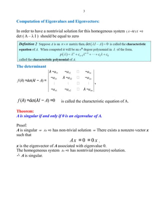
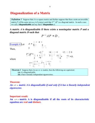
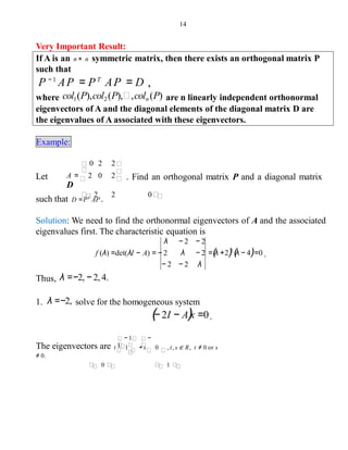
Example:
0
Let A=
1
0
0 3
0 -1 . Find the eigenvalues and eigenvectors of
A
1 3
Answer:
0
0 -1
0 1 3 z
λ z
→ - λ x +3z =0
→ x - λy - z =0
= λ y
λ x
y
3
x
1
0
→ y +( 3- λ ) z =0
3z =λ x
x − z =λ y
y +3z =λ z
3− λ z
0
= 0 Matrix form (1)
x
0y
-λ 0
1 -λ −1
0 1
3
det C =3 - λ [(-1-λ)( -3-λ ) ]
=3- λ (3+2 λ +λ2
)
=9 +3λ +λ2
- λ3
∴ λ1 =3, λ2 =-1, λ3 =-1
Then, to find the eigenvectors
matrix (1)
( X1, X2, X3 ) , substitute λ1, λ2 , λ3 into the previous

8. 8
Diagonalization of a Matrix
A matrix A is diagonalizable if there exists a nonsingular matrix P and a
diagonal matrix D such that
P − 1
AP = D .
Example 4 Let 5
.
− 4 −
6A =
3Then,
−1
P−1
AP =
−1
−2
−4
−6 −1 −2 2 0
= =D,1 1
3
5 11
0
−1
where
− 1 −
21 1
, P =
0 −
1
2 0
D =
Theorem:
An n× n matrix A is diagonalizable if and only if it has n linearly independent
eigenvector.
Important result:
An n× n matrix A is diagonalizable if all the roots of its characteristic
equation are real and distinct.

9. 9
Example 5
Let A =
.3 5
− 4 −
6
Find the nonsingular matrix P and the diagonal matrix D such that D = P − 1
AP
and find An
, n is any positive integer.
Solution:
We need to find the eigenvalues and eigenvectors of A first. The characteristic
equation of A is
=(λ +1)(λ − 2)=0.
λ +4 6
det(λI − A) =
− 3 λ − 5
λ =−1 or 2 .
By the above important result, A is diagonalizable. Then,
1. λ =2 ,
Ax =2x ⇔ (2I − A)x =0 ⇔ x =r
−1
, r ∈
R.
1
2. λ =−1,
Ax =−x ⇔ (−I − A)x =0 ⇔ x =t
−2
, t∈
R.
1
Thus, and are two linearly independent eigenvectors
of A.
1
−
1 1
−
2
Let
1
and
−1 −
2P =
1Then, by the above theorem,
−
1 .
2 0
D =
0
D = P −1
AP .

10. 10
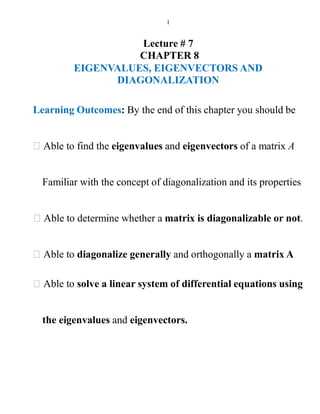
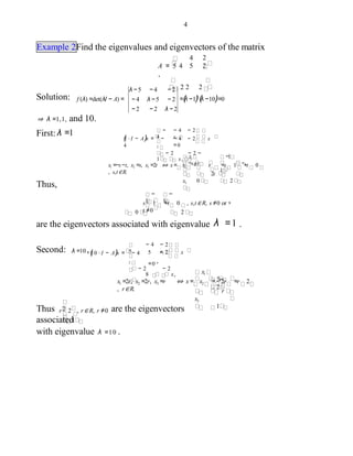
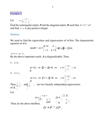
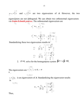
To find An
,
D = =(P AP)(P AP) (P AP)=P A P
0 (−1)n
−1 −1 −1 −1 n2n
0n
Multiplied by P and P−1
on the both sides,
(−1)n
1
− [2n
+2⋅(−1)n+1
] − [2n+1
+2⋅(−1)n+1
]
2n
+(−1)n+1
2n+1
+(−1)n+1
=
1
−1
−
2
1
0
−
2
2
= =
1
−
1PDn
P−1
=
−1
PP−1
An
PP−1
An 0n
Note (very important):
If A is an n × n diagonalizable matrix, then there exists an nonsingular matrix
P such that
D = P −1
AP ,
where col1(P), col2 (P), , coln (P) are n linearly independent eigenvectors of
A and the diagonal elements of the diagonal matrix D are the eigenvalues of A
associated with these eigenvectors.
Note:
For any n × n diagonalizable matrix A, D = P − 1
A P ,
then
=PDk
P−1
, k =1,2,Ak
where
λk.
λk
0 0
λ2 0
0 0
D k
=
0
n
k
1

11. 11
Example:
Is A =
diagonalizable?3 −
1
5 −
3
Solution: =(λ − 2)2
=0
− 3 λ +1
λ − 5 3
det(λI − A) =
Then, λ = 2, 2 .
λ =2, (2I − A)x = 0
1
⇔ x = t , t ∈ R.
1
Therefore, all the eigenvectors are spanned by . There does not exist
two
1
linearly independent eigenvectors. By the previous theorem, A is not
diagonalizable.
1
Note:
An n× n matrix may fail to be diagonalizable since
1. Not all roots of its characteristic equation are real numbers.
2. It does not have n linearly independent eigenvectors.
Note:
Definition: The set S j consisting of both all eigenvectors of an n× n matrix A
associated with eigenvalue λj and zero vector 0 is a subspace of R . S is calledn
j
the eigenspace associated with λj .

12. 12
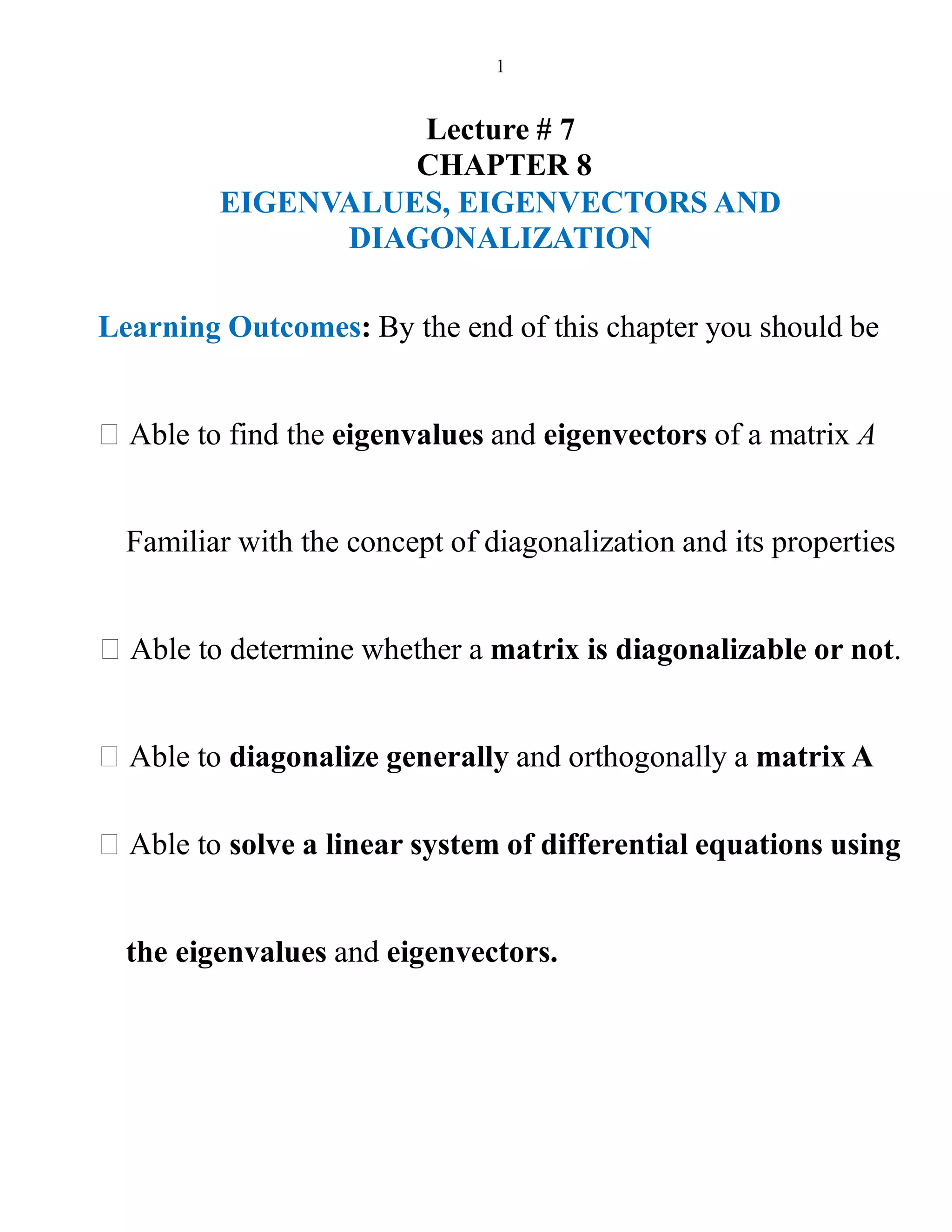
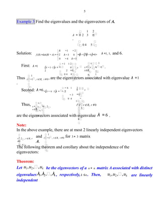
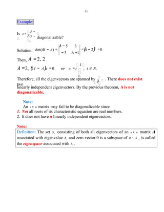
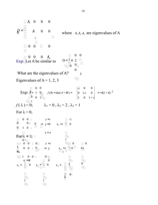
Diagonalization of Symmetric Matrix
Theorem:
If A is an n× n symmetric matrix, then the eigenvectors of A associated with
distinct eigenvalues are orthogonal.
[proof:]
Let x1 =
a2
an bn
a1
and x2 =
b2
b1
be eigenvectors of A associated with distinct
eigenvalues λ1 and λ2 , respectively, i.e., Ax1 = λ1 x1 and Ax2 =λ2 x2 .
Thus, x1 Ax2 =x1 (Ax2 )=x1λ2x2 =λ2x1x2 andt t t t
xt
Ax =xt
At
x =(xt
At
)x =(Ax )t
x =(λ x )t
x =λ xt
x .1 2 1 2 1 2 1 2 1 1 2 1 1 2
Therefore, xt
Ax =λ xt
x =λ xt
x .1 2 2 1 2 1 1 2
Since λ1 ≠ λ2 , x 1 x 2 =
0 .
t
Example:
Let A =
0
0
− 2 0
− 20 3
−
20
A is a symmetric matrix. The characteristic equation is
λ 0 2
λ+2 0 =(λ+2)(λ− 4)(λ+1)=0 .
2 0 λ− 3
det(λI − A) =0
The eigenvalues of A are − 2, 4, − 1. The eigenvectors associated with these
eigenvalues are
0 −1 2
x1 = 1 (λ =2), x2 = 0 (λ =4), x3 = 0 (λ
=−1).
1
2
0
Thus, x1,x2,x3 are orthogonal.

13. 13
Definition of an orthogonal matrix:
An n× nnonsingular matrix A is called an orthogonal matrix if A−1
=AT
Intuition:
col1 (
A )=
col2 (
A )
colT
(A )
( ) ( ) (
)
col1 (A )col1 (
A )
col1 (A )col2 (A ) col1 (A )coln (
A )=
col2 (A )col1 (
A )
col2 (A )col2 (A ) col2 (A )col (
A )
coln (A )col1 (
A )
coln (A )col2 (A ) coln (A )coln (
A )
col1
A
col2 A col A
T
T
T
n
n
T T T
T T T
n
T T T
A
A
col1 (A )⋅ col1 (
A )
col2 (A )⋅ col1 (
A )
=
col1 (A )⋅ col2 (A )
col2 (A )⋅ col2 (A )
coln (A )⋅ col2 (A )
col1 (A )⋅ coln (A )
col2 (A )⋅ coln (
A )
coln (A )⋅ col1 (
A )
coln (A )⋅ coln (
A )1 0
0
0 1
0
0 0
1
=
I
n
=
col (A)⋅col (A)= col (A)2
=1,
i i i
coli (A)⋅colj (A)=0, i ≠ j
That is, all of column vectors of A are orthonormal.
Important Result:
An n× n matrix A is orthogonal if and only if the columns (or rows) of A form
an orthonormal set of vectors.
i =1, 2, ,n

14. 14
Very Important Result:
If A is an n× n symmetric matrix, then there exists an orthogonal matrix P
such that
P − 1
AP = PT
AP = D ,
where col1(P),col2(P), ,coln (P) are n linearly independent orthonormal
eigenvectors of A and the diagonal elements of the diagonal matrix D are
the eigenvalues of A associated with these eigenvectors.
Example:
Let
0 2 2
A = 2 0 2 . Find an orthogonal matrix P and a diagonal matrix
D
2 2 0
such that D =PT
AP .
Solution: We need to find the orthonormal eigenvectors of A and the associated
eigenvalues first. The characteristic equation is
λ − 2 − 2
λ − 2 =(λ +2)2
(λ − 4)=0 .
− 2 − 2 λ
f (λ) =det(λI − A) = − 2
Thus, λ =−2, − 2, 4.
1. λ =−2, solve for the homogeneous system
(− 2I − A)x =0.
The eigenvectors are t 1 + s 0 , t, s ∈ R, t ≠ 0 or s
≠ 0.
0 1
− 1 −
1

15. 15
0
⇒ v = 1
−
1
1 and v
1
= 0
−
1
2 are two eigenvectors of A. However, the two
eigenvectors are not orthogonal. We can obtain two orthonormal eigenvectors
via Gram-Schmidt process. The orthonormal eigenvectors are
− 1
= − 1/
2
− 1/
2 .
v ⋅
v
−
v2 ⋅ v1
v
v*
=v
2 2 0
= 1v*
=v
1 1
1
1
1 1
Standardizing these two eigenvectors results in
− 1 /
− 1 / 6
= − 1 / 6
62 /
w 2
=
.
2
= 1 / 2w 1
= 0
2
*
v 2
v *
1
*
v 1
v *
2. λ =4, solve for the homogeneous system (4I − A)x =0.
1
The eigenvectors are r 1 , r ∈ R, r ≠
0 .
1
1v3 = 1 is an eigenvectors of A. Standardizing the eigenvector results
in
1
3
Thus,
1 / 3
= 1 / 3
.
1 /
w =
3
3
3
v
v

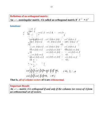
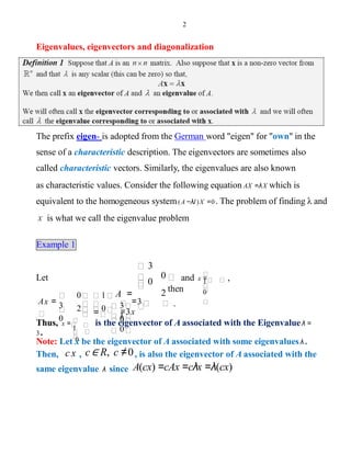
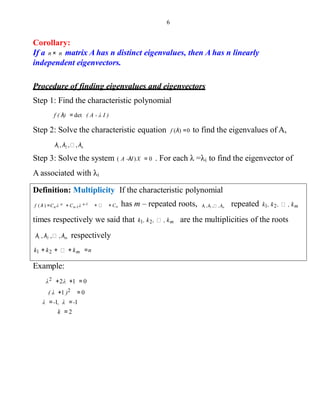
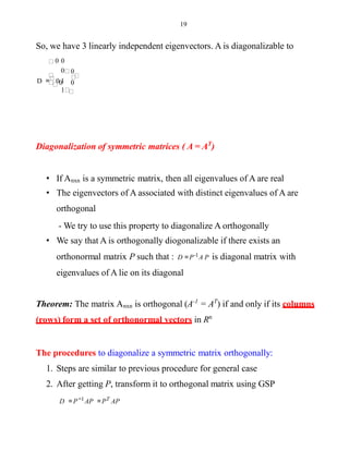
16. 16
P =[w1
diagonalizable?)
w2 w3 ]=
1/ 3
1/
3
,
3−1/ 2 −1/ 6 1/
2 −1/ 6
0 2/ 6 1/
− 2 0 0
− 2 0
0 0 4,
D =
0
and D =PT
AP .
Summary
What is diagonalization? To answer this let see what are similar matrices
We said that B is similar to A if there exists a matrix P such that B = P-1
A P
1. A is similar to A
2. If B is similar to A, then A is similar to B
3. If B is similar to A and A is similar to C. Then, B is similar to C.
** Similar matrices have same eigenvalues
** A matrix Amxn is diagonalizable if it is similar to a matrix D =P
where
P is the matrix whose columns are the eigenvectors of A.
A P−1
λn
2
λ1
D =
λ
Where λ , λ , λ are the eigenvalues of A1 2 n
Is every matrix diagonalizable? (Or what are the conditions for a matrix A to be

17. 17
Theorem: A matrix Anxn is diagonalizable if and only if it has an n-linearly
independent eigenvectors.
We know that a matrix with a distinct eigenvalues will has n-linearly
independent eigenvectors. So:
Theorem: If a matrix Anxn has n distinct eigenvalues, then it is diagonalizable.
**This does not mean that if it has m < n distinct eigenvalues, then it is not
diagonalizable.
So, how can we diagonalize it?
Procedure to diagonalize a matrix A (p.428)
Step 1: Find eigenvalues of A. check if all eigenvalues are distinct. Then A is
diagonalizable
λn
2
λ1
D =
λ
Step 2: If there is eigenvalues λj with multiplicity kj, Check the dimension of
solution space of (A - λ j I)X =0 . If dim SS = kj, then A is diagonalizable –go step
3 - otherwise the matrix is not diagonalizable.
Step 3: find the eigenvectors X1,X 2 , ,X n of A
Step 4: Write D =P-1
A P , where P =[X1,X2, ,Xn ]

18. 18
λ1 0 0 0
λ 0 0
2
0 0 0
0 0 0 λn
D =
0 where λ1, λ2 , λn are eigenvalues of A
Exp: Let A be similar to
0
D = 0 2
0
0
3
0
0
What are the eigenvalues of A?
Eigenvalues of A = 1, 2, 3
1
Exp: A =
0
1
00
1 0 f (λ) =det(A− λI) =
0 1
0
-λ 0 0
0 1-λ 0
1 0 1− λ
2
=−λ(1− λ)
f ( λ ) = 0;
For λ = 0,
λ1 = 0 , λ2 = 2 , λ3 = 1
1
z =r
⇒ y =0 x =r 0
x =-r
-10 0 :
0
1 0 :
1 0 1 :
0
0
0
0
1
For λ = 1,
0
x =r 0 + s
1
0
1
0
00 0 : 0 z =r
0 0 : ⇒ y
=s
1 0 0 : 0
x =0
0
0
-
1
2
1
0
x =
1
= 0
0
1
0
-1
x = x 321

19. 19
So, we have 3 linearly independent eigenvectors. A is diagonalizable to
0 0
1
0
0 0
0
D = 0 1
Diagonalization of symmetric matrices ( A = AT
)
• If Anxn is a symmetric matrix, then all eigenvalues of A are real
• The eigenvectors of A associated with distinct eigenvalues of A are
orthogonal
- We try to use this property to diagonalize A orthogonally
• We say that A is orthogonally diogonalizable if there exists an
orthonormal matrix P such that : D =P-1A P is diagonal matrix with
eigenvalues of A lie on its diagonal
Theorem: The matrix Anxn is orthogonal (A-1
= AT
) if and only if its columns
(rows) form a set of orthonormal vectors in Rn
The procedures to diagonalize a symmetric matrix orthogonally:
1. Steps are similar to previous procedure for general case
2. After getting P, transform it to orthogonal matrix using GSP
D = P−1AP =PT AP

20. 20
Since, P is orthogonal
Suppose that we have n-distinct eigenvalues. Then, we have n-linearly
independent eigenvectors.
∀i ,jx1, x2, , xn so xi • x j = 0
P =[x1, x2, , xn ] transformit intoorthogonal matrix
→ P = 1 , 2 , , n
xn
x1
x
x
x2
x
Otherwise we need to go through GSP
2
Example: Let A = 2 0
2
2 2 0
2
0
- λ 2 2
2 − λ 2
2 2 − λ
f (λ ) =det (A- λ I ) = = ( λ – 4) (λ + 2)2
λ1 =
4,
λ2 = λ3 = -2
For λ = 4,
1
1
1
∴ x = r
x =r
y =r
: 0 z =r
0
01 1 :
1 -1 :
0 0
0
0
-
2→
2 2 :
-4 2 :
22 -4 :
0
0
0
2
-
4
1
For λ = -2,
0
s
−
1+
1
r 0
-1
x =
z =r
y =s
0 x =-r - s
0
01 1 :
0 0 :
0 0
0 :
0
1→
2 2 :
2 2 :
2 2 2 :
0
0
0
2
2 12
, x3 = 1
0
−
1∴ x2 = 0
1
-1
P = [ x1 x2 x3 ],
4 0 0
-2 0
0 0 -2
D = 0
Examples (p.456-457)