Linear algebra: matrix Eigen-value
Problems
Eng. Shubham Kumbhar
Part 3
Eigenvalue Problems
1. Eigenvalues and eigenvectors
2. Vector spaces
3. Linear transformations
4. Matrix diagonalization
The Eigenvalue Problem
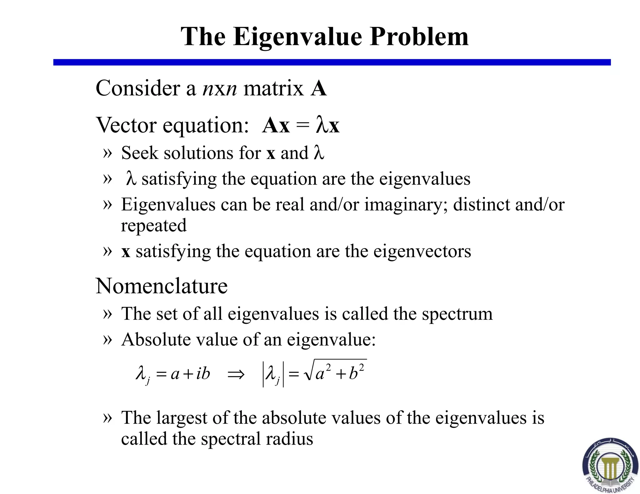
Consider a nxn matrix A
Vector equation: Ax = λx
» Seek solutions for x and λ
» λ satisfying the equation are the eigenvalues
» Eigenvalues can be real and/or imaginary; distinct and/or
repeated
» x satisfying the equation are the eigenvectors
Nomenclature
» The set of all eigenvalues is called the spectrum
» Absolute value of an eigenvalue:
» The largest of the absolute values of the eigenvalues is
called the spectral radius
22
baiba jj +=⇒+= λλ
Determining Eigenvalues
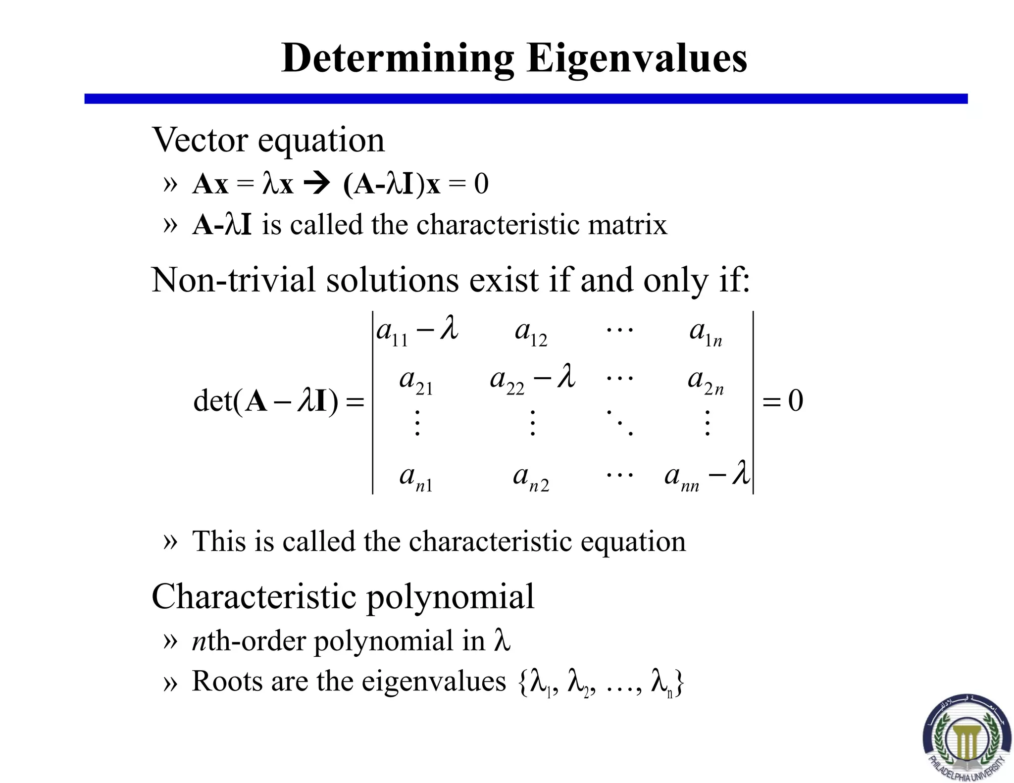
Vector equation
» Ax = λx  (A-λΙ)x = 0
» A-λΙ is called the characteristic matrix
Non-trivial solutions exist if and only if:
» This is called the characteristic equation
Characteristic polynomial
» nth-order polynomial in λ
» Roots are the eigenvalues {λ1, λ2, …, λn}
0)det(
21
22221
11211
=
−
−
−
=−
λ
λ
λ
λ
nnnn
n
n
aaa
aaa
aaa




IA
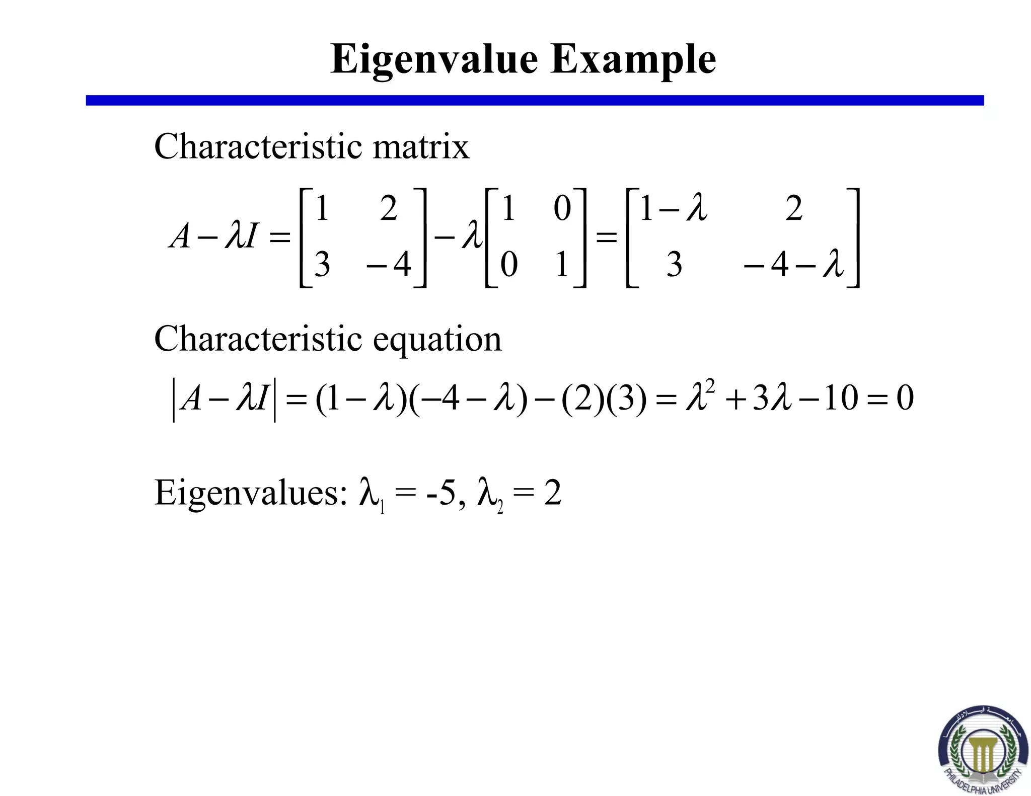
Eigenvalue Example
Characteristic matrix
Characteristic equation
Eigenvalues: λ1 = -5, λ2 = 2






−−
−
=





−





−
=−
λ
λ
λλ
43
21
10
01
43
21
IA
0103)3)(2()4)(1( 2
=−+=−−−−=− λλλλλIA
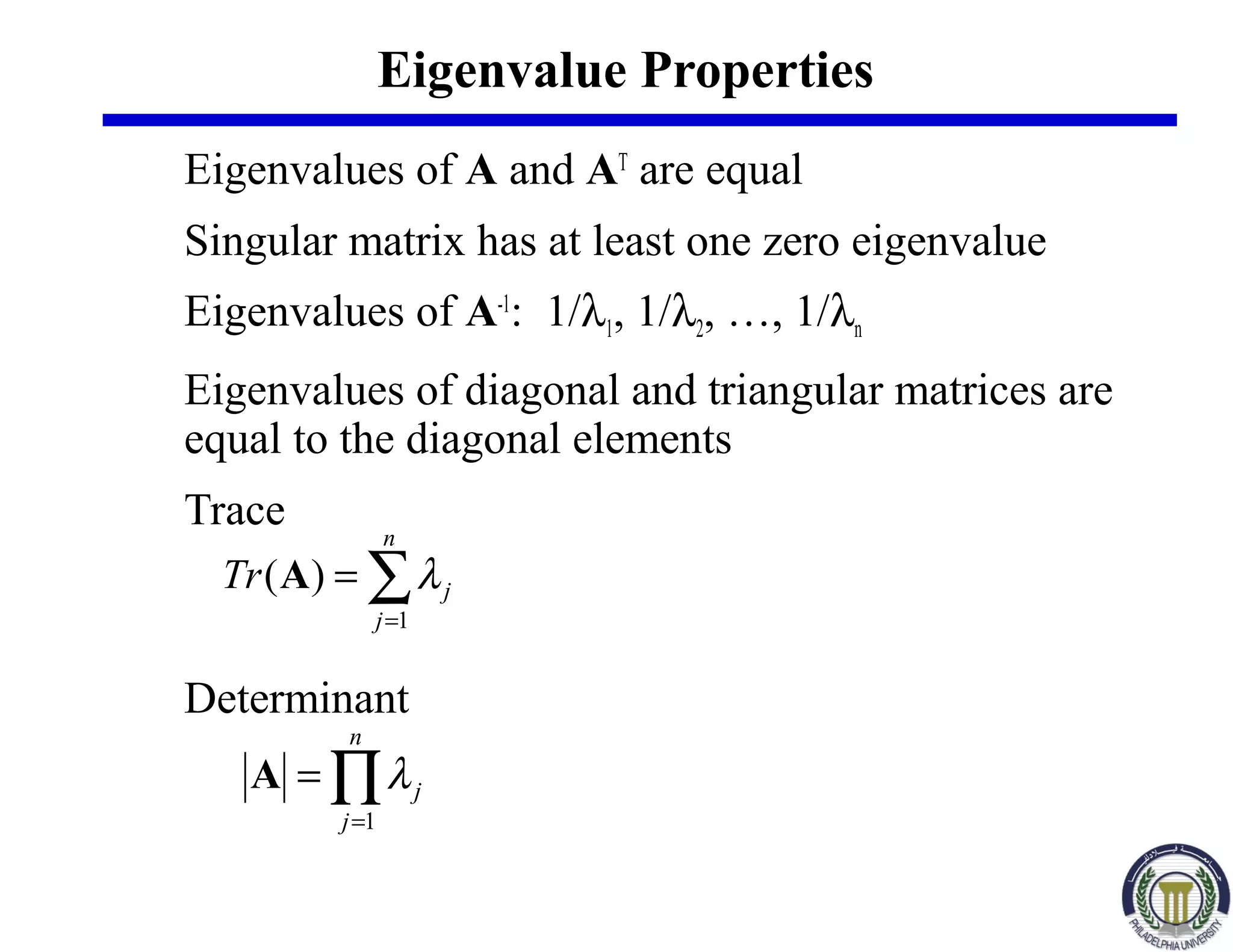
Eigenvalue Properties
Eigenvalues of A and AT
are equal
Singular matrix has at least one zero eigenvalue
Eigenvalues of A-1
: 1/λ1, 1/λ2, …, 1/λn
Eigenvalues of diagonal and triangular matrices are
equal to the diagonal elements
Trace
Determinant
∑=
=
n
j
jTr
1
)( λA
∏=
=
n
j
j
1
λA
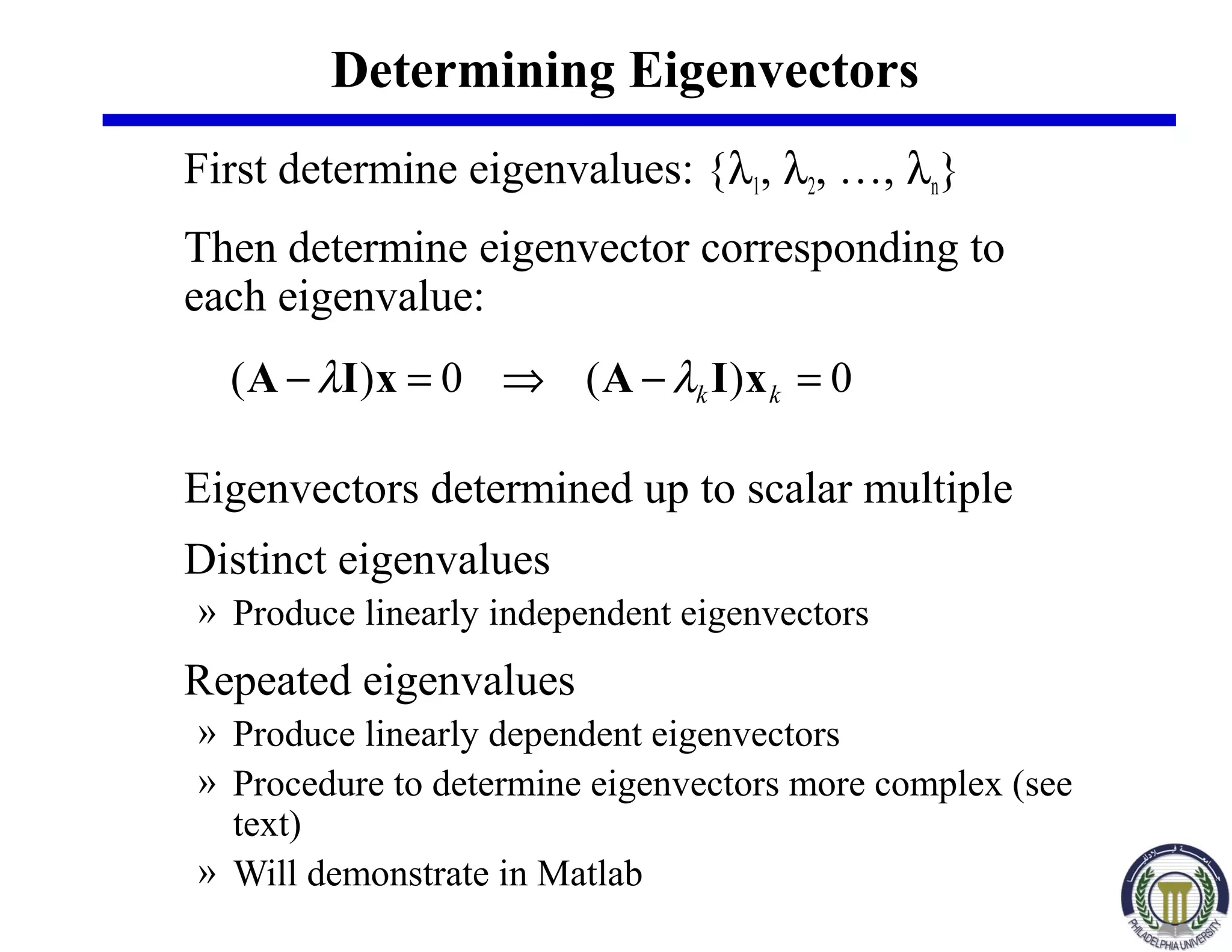
Determining Eigenvectors
First determine eigenvalues: {λ1, λ2, …, λn}
Then determine eigenvector corresponding to
each eigenvalue:
Eigenvectors determined up to scalar multiple
Distinct eigenvalues
» Produce linearly independent eigenvectors
Repeated eigenvalues
» Produce linearly dependent eigenvectors
» Procedure to determine eigenvectors more complex (see
text)
» Will demonstrate in Matlab
0)(0)( =−⇒=− kk xIAxIA λλ
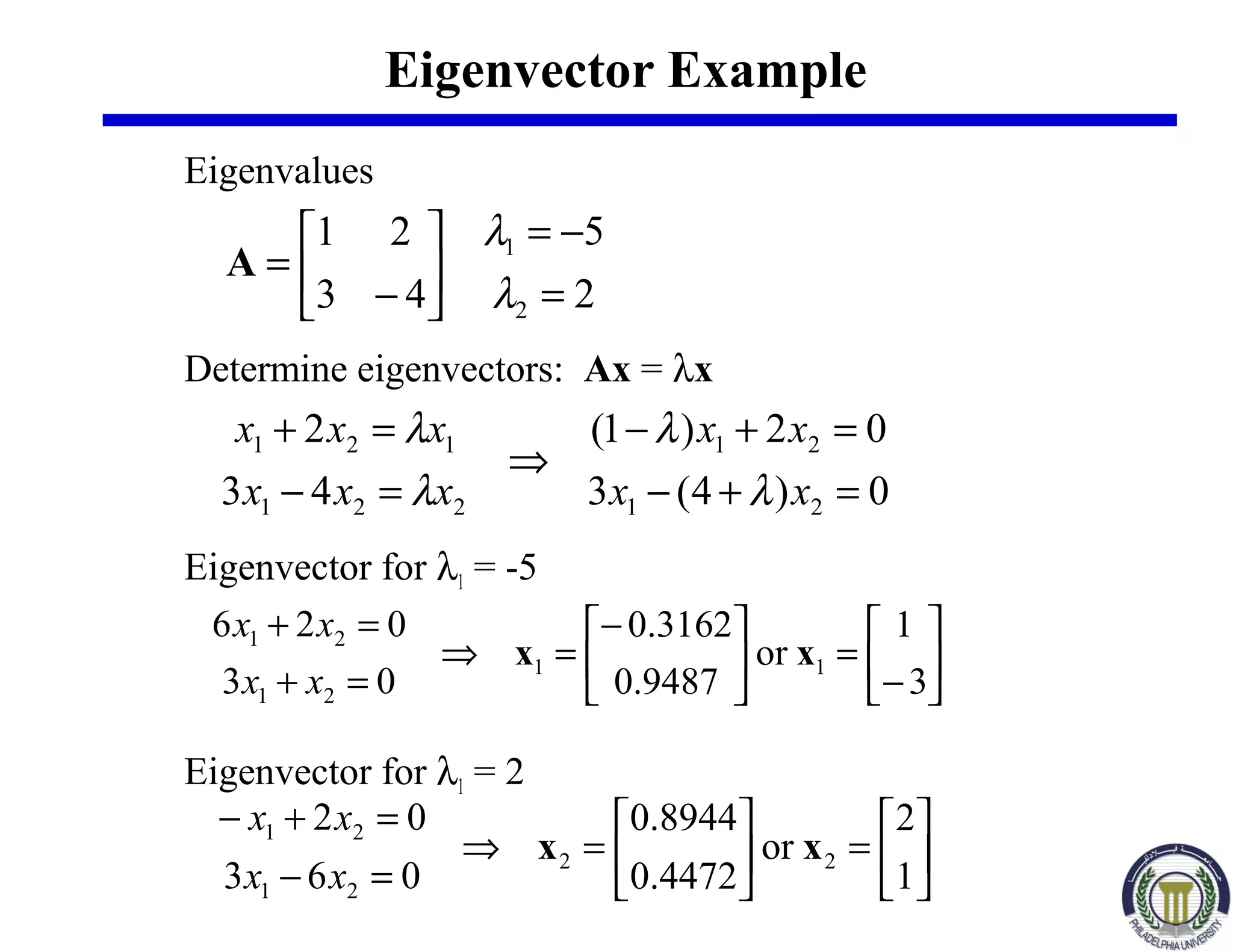
Eigenvector Example
Eigenvalues
Determine eigenvectors: Ax = λx
Eigenvector for λ1 = -5
Eigenvector for λ1 = 2






−
=




−
=⇒
=+
=+
3
1
or
9487.0
3162.0
03
026
11
21
21
xx
xx
xx






=





=⇒
=−
=+−
1
2
or
4472.0
8944.0
063
02
22
21
21
xx
xx
xx
2
5
43
21
2
1
=
−=






−
=
λ
λ
A
0)4(3
02)1(
43
2
21
21
221
121
=+−
=+−
⇒
=−
=+
xx
xx
xxx
xxx
λ
λ
λ
λ
Matlab Examples
>> A=[ 1 2; 3 -4];
>> e=eig(A)
e =
2
-5
>> [X,e] = eig(A)
X =
0.8944 -0.3162
0.4472 0.9487
e =
2 0
0 -5
>> A=[2 5; 0 2];
>> e=eig(A)
e =
2
2
>> [X,e]=eig(A)
X =
1.0000 -1.0000
0 0.0000
e =
2 0
0 2
Vector Spaces
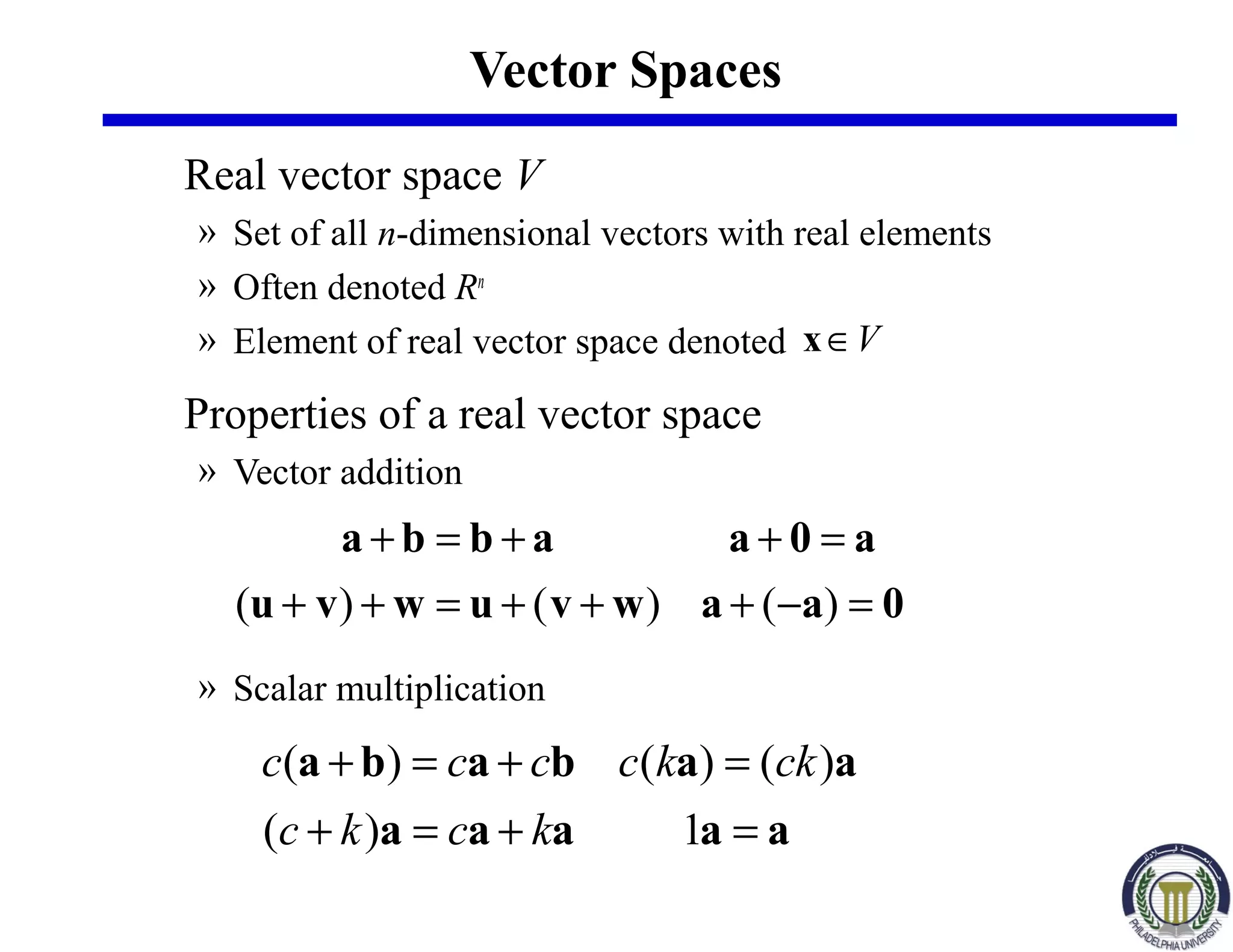
Real vector space V
» Set of all n-dimensional vectors with real elements
» Often denoted Rn
» Element of real vector space denoted
Properties of a real vector space
» Vector addition
» Scalar multiplication
V∈x
0aawvuwvu
a0aabba
=−+++=++
=++=+
)()()(
aaaaa
aababa
=+=+
=+=+
1)(
)()()(
kckc
ckkcccc
Vector Spaces cont.
Linearly independent vectors
» Elements:
» Linear combination:
» Equation satisfied only for cj = 0
Basis
» n-dimensional vector space V contains exactly n linearly
independent vectors
» Any n linearly independent vectors form a basis for V
» Any element of V can be expressed as a linear
combination of the basis vectors
Example: unit basis vectors in R3
021 =+++ (m)(2)(1) aaa mccc 
V∈(m)(2)(1) aaa ,,, 










=










+










+










=++=
3
2
1
3213321
1
0
0
0
1
0
0
0
1
c
c
c
cccccc )((2)(1) aaax
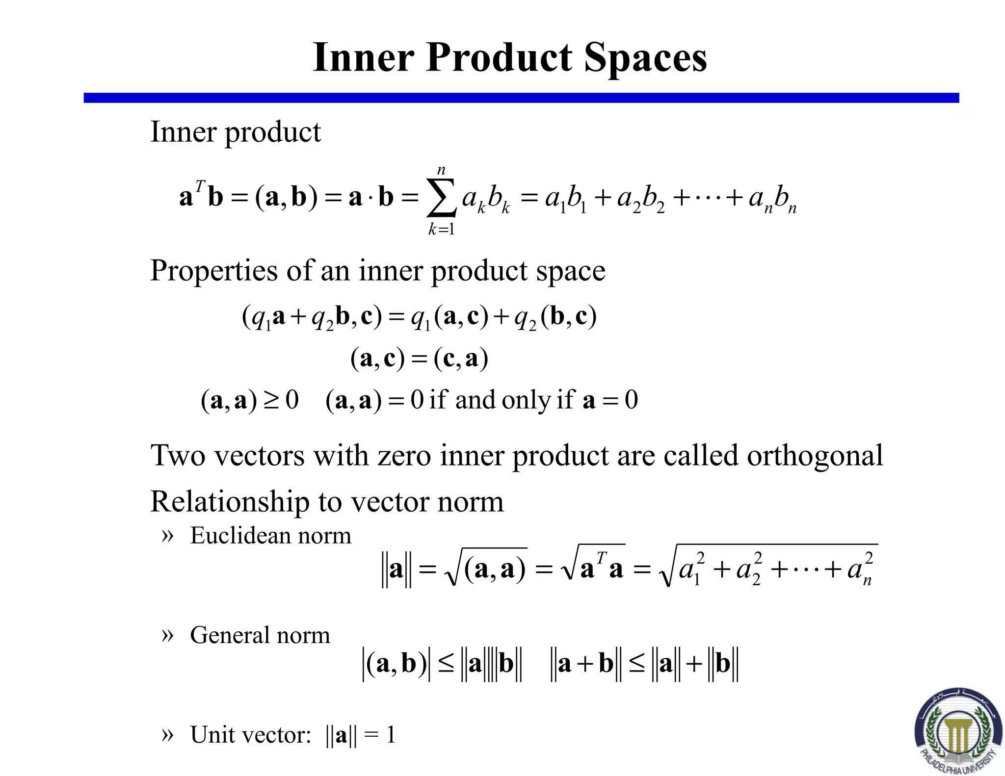
Inner Product Spaces
Inner product
Properties of an inner product space
Two vectors with zero inner product are called orthogonal
Relationship to vector norm
» Euclidean norm
» General norm
» Unit vector: ||a|| = 1
∑=
+++==⋅==
n
k
nnkk
T
babababa
1
2211),( bababa
0ifonlyandif0),(0),(
),(),(
),(),(),( 2121
==≥
=
+=+
aaaaa
acca
cbcacba qqqq
22
2
2
1),( n
T
aaa +++=== aaaaa
babababa +≤+≤),(
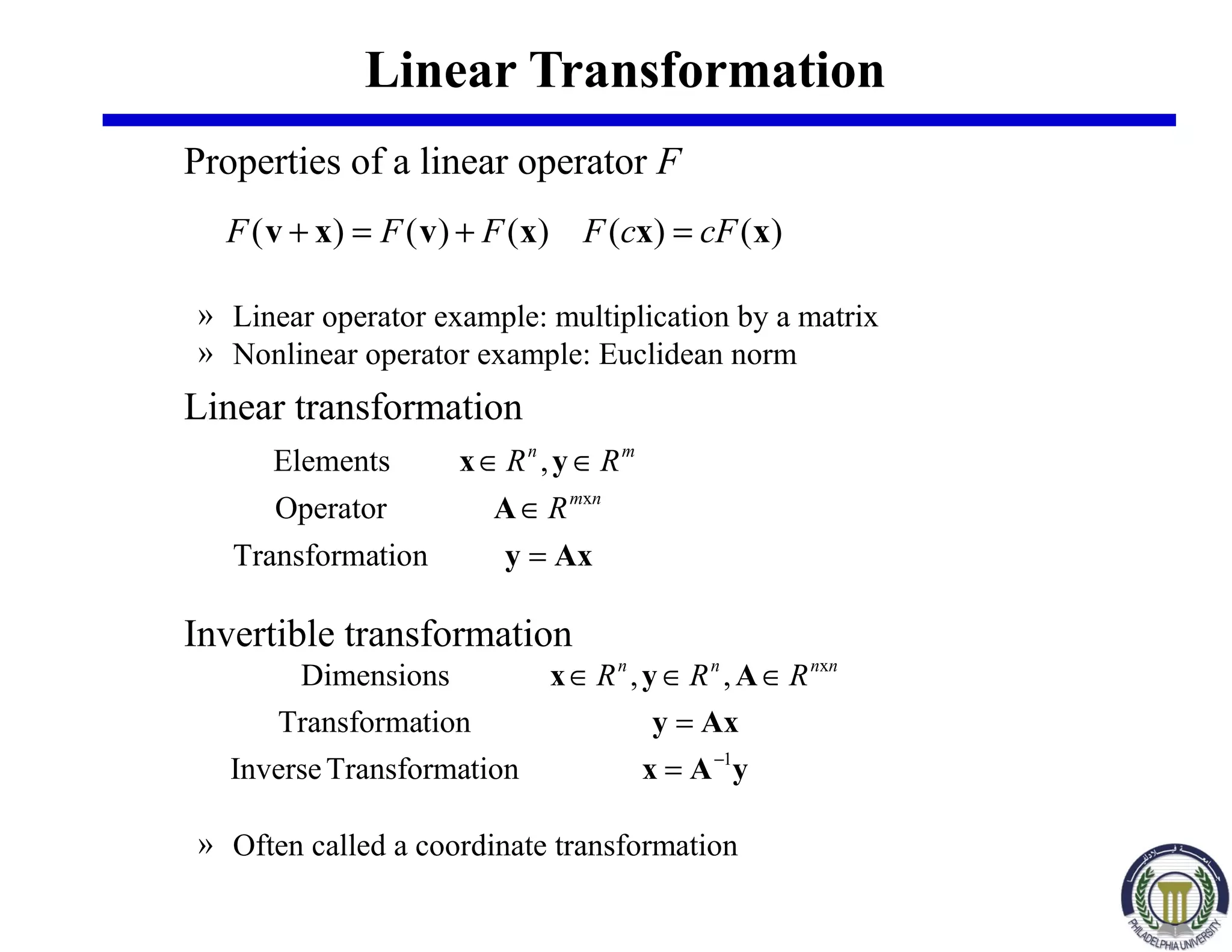
Linear Transformation
Properties of a linear operator F
» Linear operator example: multiplication by a matrix
» Nonlinear operator example: Euclidean norm
Linear transformation
Invertible transformation
» Often called a coordinate transformation
)()()()()( xxxvxv cFcFFFF =+=+
Axy
A
yx
=
∈
∈∈
tionTransforma
Operator
,Elements
xnm
mn
R
RR
yAx
Axy
Ayx
1
x
tionTransformaInverse
tionTransforma
,,Dimensions
−
=
=
∈∈∈ nnnn
RRR
Orthogonal Transformations
Orthogonal matrix
» A square matrix satisfying: AT
= A-1
» Determinant has value +1 or -1
» Eigenvalues are real or complex conjugate pairs with
absolute value of unity
» A square matrix is orthonormal if:
Orthogonal transformation
» y = Ax where A is an orthogonal matrix
» Preserves the inner product between any two vectors
» The norm is also invariant to orthogonal transformation
bavuAbvAau ⋅=⋅⇒== ,



=
≠
=
kj
kj
k
T
j
if1
if0
aa
vbua ==
Similarity Transformations
Eigenbasis
» If a nxn matrix has n distinct eigenvalues, the
eigenvectors form a basis for Rn
» The eigenvectors of a symmetric matrix form an
orthonormal basis for Rn
» If a nxn matrix has repeated eigenvalues, the
eigenvectors may not form a basis for Rn
(see text)
Similar matrices
» Two nxn matrices are similar if there exists a
nonsingular nxn matrix P such that:
» Similar matrices have the same eigenvalues
» If x is an eigenvector of A, then y = P-1
x is an
eigenvector of the similar matrix
APPA 1ˆ −
=
Matrix Diagonalization
Assume the nxn matrix A has an eigenbasis
Form the nxn modal matrix X with the eigenvectors
of A as column vectors: X = [x1, x2, …, xn]
Then the similar matrix D = X-1
AX is diagonal with
the eigenvalues of A as the diagonal elements
Companion relation: XDX-1
= A












==⇒












= −
nnnnn
n
n
aaa
aaa
aaa
λ
λ
λ








00
00
00
2
1
1
21
22221
11211
AXXDA
Matrix Diagonalization Example
[ ]





−
=




−





 −
==






−





−




 −
==





 −
=





−
==






==





−
=−=





−
=
−
−
−
20
05
215
45
13
21
7
1
13
21
43
21
13
21
7
1
13
21
7
1
13
21
1
2
,2
3
1
,5
43
21
1
1
1
21
2211
AXXD
AXXD
XxxX
xxA λλ
Matlab Example
>> A=[-1 2 3; 4 -5 6; 7 8 -9];
>> [X,e]=eig(A)
X =
-0.5250 -0.6019 -0.1182
-0.5918 0.7045 -0.4929
-0.6116 0.3760 0.8620
e =
4.7494 0 0
0 -5.2152 0
0 0 -14.5343
>> D=inv(X)*A*X
D =
4.7494 -0.0000 -0.0000
-0.0000 -5.2152 -0.0000
0.0000 -0.0000 -14.5343

Eigen values and eigen vectors engineering

  • 1.
    Linear algebra: matrixEigen-value Problems Eng. Shubham Kumbhar Part 3
  • 2.
    Eigenvalue Problems 1. Eigenvaluesand eigenvectors 2. Vector spaces 3. Linear transformations 4. Matrix diagonalization
  • 3.
    The Eigenvalue Problem Considera nxn matrix A Vector equation: Ax = λx » Seek solutions for x and λ » λ satisfying the equation are the eigenvalues » Eigenvalues can be real and/or imaginary; distinct and/or repeated » x satisfying the equation are the eigenvectors Nomenclature » The set of all eigenvalues is called the spectrum » Absolute value of an eigenvalue: » The largest of the absolute values of the eigenvalues is called the spectral radius 22 baiba jj +=⇒+= λλ
  • 4.
    Determining Eigenvalues Vector equation »Ax = λx  (A-λΙ)x = 0 » A-λΙ is called the characteristic matrix Non-trivial solutions exist if and only if: » This is called the characteristic equation Characteristic polynomial » nth-order polynomial in λ » Roots are the eigenvalues {λ1, λ2, …, λn} 0)det( 21 22221 11211 = − − − =− λ λ λ λ nnnn n n aaa aaa aaa     IA
  • 5.
    Eigenvalue Example Characteristic matrix Characteristicequation Eigenvalues: λ1 = -5, λ2 = 2       −− − =      −      − =− λ λ λλ 43 21 10 01 43 21 IA 0103)3)(2()4)(1( 2 =−+=−−−−=− λλλλλIA
  • 6.
    Eigenvalue Properties Eigenvalues ofA and AT are equal Singular matrix has at least one zero eigenvalue Eigenvalues of A-1 : 1/λ1, 1/λ2, …, 1/λn Eigenvalues of diagonal and triangular matrices are equal to the diagonal elements Trace Determinant ∑= = n j jTr 1 )( λA ∏= = n j j 1 λA
  • 7.
    Determining Eigenvectors First determineeigenvalues: {λ1, λ2, …, λn} Then determine eigenvector corresponding to each eigenvalue: Eigenvectors determined up to scalar multiple Distinct eigenvalues » Produce linearly independent eigenvectors Repeated eigenvalues » Produce linearly dependent eigenvectors » Procedure to determine eigenvectors more complex (see text) » Will demonstrate in Matlab 0)(0)( =−⇒=− kk xIAxIA λλ
  • 8.
    Eigenvector Example Eigenvalues Determine eigenvectors:Ax = λx Eigenvector for λ1 = -5 Eigenvector for λ1 = 2       − =     − =⇒ =+ =+ 3 1 or 9487.0 3162.0 03 026 11 21 21 xx xx xx       =      =⇒ =− =+− 1 2 or 4472.0 8944.0 063 02 22 21 21 xx xx xx 2 5 43 21 2 1 = −=       − = λ λ A 0)4(3 02)1( 43 2 21 21 221 121 =+− =+− ⇒ =− =+ xx xx xxx xxx λ λ λ λ
  • 9.
    Matlab Examples >> A=[1 2; 3 -4]; >> e=eig(A) e = 2 -5 >> [X,e] = eig(A) X = 0.8944 -0.3162 0.4472 0.9487 e = 2 0 0 -5 >> A=[2 5; 0 2]; >> e=eig(A) e = 2 2 >> [X,e]=eig(A) X = 1.0000 -1.0000 0 0.0000 e = 2 0 0 2
  • 10.
    Vector Spaces Real vectorspace V » Set of all n-dimensional vectors with real elements » Often denoted Rn » Element of real vector space denoted Properties of a real vector space » Vector addition » Scalar multiplication V∈x 0aawvuwvu a0aabba =−+++=++ =++=+ )()()( aaaaa aababa =+=+ =+=+ 1)( )()()( kckc ckkcccc
  • 11.
    Vector Spaces cont. Linearlyindependent vectors » Elements: » Linear combination: » Equation satisfied only for cj = 0 Basis » n-dimensional vector space V contains exactly n linearly independent vectors » Any n linearly independent vectors form a basis for V » Any element of V can be expressed as a linear combination of the basis vectors Example: unit basis vectors in R3 021 =+++ (m)(2)(1) aaa mccc  V∈(m)(2)(1) aaa ,,,            =           +           +           =++= 3 2 1 3213321 1 0 0 0 1 0 0 0 1 c c c cccccc )((2)(1) aaax
  • 12.
    Inner Product Spaces Innerproduct Properties of an inner product space Two vectors with zero inner product are called orthogonal Relationship to vector norm » Euclidean norm » General norm » Unit vector: ||a|| = 1 ∑= +++==⋅== n k nnkk T babababa 1 2211),( bababa 0ifonlyandif0),(0),( ),(),( ),(),(),( 2121 ==≥ = +=+ aaaaa acca cbcacba qqqq 22 2 2 1),( n T aaa +++=== aaaaa babababa +≤+≤),(
  • 13.
    Linear Transformation Properties ofa linear operator F » Linear operator example: multiplication by a matrix » Nonlinear operator example: Euclidean norm Linear transformation Invertible transformation » Often called a coordinate transformation )()()()()( xxxvxv cFcFFFF =+=+ Axy A yx = ∈ ∈∈ tionTransforma Operator ,Elements xnm mn R RR yAx Axy Ayx 1 x tionTransformaInverse tionTransforma ,,Dimensions − = = ∈∈∈ nnnn RRR
  • 14.
    Orthogonal Transformations Orthogonal matrix »A square matrix satisfying: AT = A-1 » Determinant has value +1 or -1 » Eigenvalues are real or complex conjugate pairs with absolute value of unity » A square matrix is orthonormal if: Orthogonal transformation » y = Ax where A is an orthogonal matrix » Preserves the inner product between any two vectors » The norm is also invariant to orthogonal transformation bavuAbvAau ⋅=⋅⇒== ,    = ≠ = kj kj k T j if1 if0 aa vbua ==
  • 15.
    Similarity Transformations Eigenbasis » Ifa nxn matrix has n distinct eigenvalues, the eigenvectors form a basis for Rn » The eigenvectors of a symmetric matrix form an orthonormal basis for Rn » If a nxn matrix has repeated eigenvalues, the eigenvectors may not form a basis for Rn (see text) Similar matrices » Two nxn matrices are similar if there exists a nonsingular nxn matrix P such that: » Similar matrices have the same eigenvalues » If x is an eigenvector of A, then y = P-1 x is an eigenvector of the similar matrix APPA 1ˆ − =
  • 16.
    Matrix Diagonalization Assume thenxn matrix A has an eigenbasis Form the nxn modal matrix X with the eigenvectors of A as column vectors: X = [x1, x2, …, xn] Then the similar matrix D = X-1 AX is diagonal with the eigenvalues of A as the diagonal elements Companion relation: XDX-1 = A             ==⇒             = − nnnnn n n aaa aaa aaa λ λ λ         00 00 00 2 1 1 21 22221 11211 AXXDA
  • 17.
    Matrix Diagonalization Example []      − =     −       − ==       −      −      − ==       − =      − ==       ==      − =−=      − = − − − 20 05 215 45 13 21 7 1 13 21 43 21 13 21 7 1 13 21 7 1 13 21 1 2 ,2 3 1 ,5 43 21 1 1 1 21 2211 AXXD AXXD XxxX xxA λλ
  • 18.
    Matlab Example >> A=[-12 3; 4 -5 6; 7 8 -9]; >> [X,e]=eig(A) X = -0.5250 -0.6019 -0.1182 -0.5918 0.7045 -0.4929 -0.6116 0.3760 0.8620 e = 4.7494 0 0 0 -5.2152 0 0 0 -14.5343 >> D=inv(X)*A*X D = 4.7494 -0.0000 -0.0000 -0.0000 -5.2152 -0.0000 0.0000 -0.0000 -14.5343