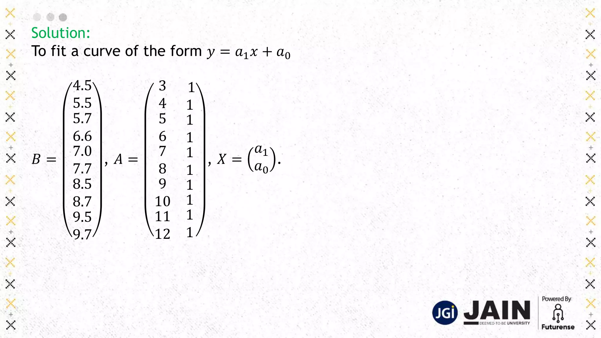
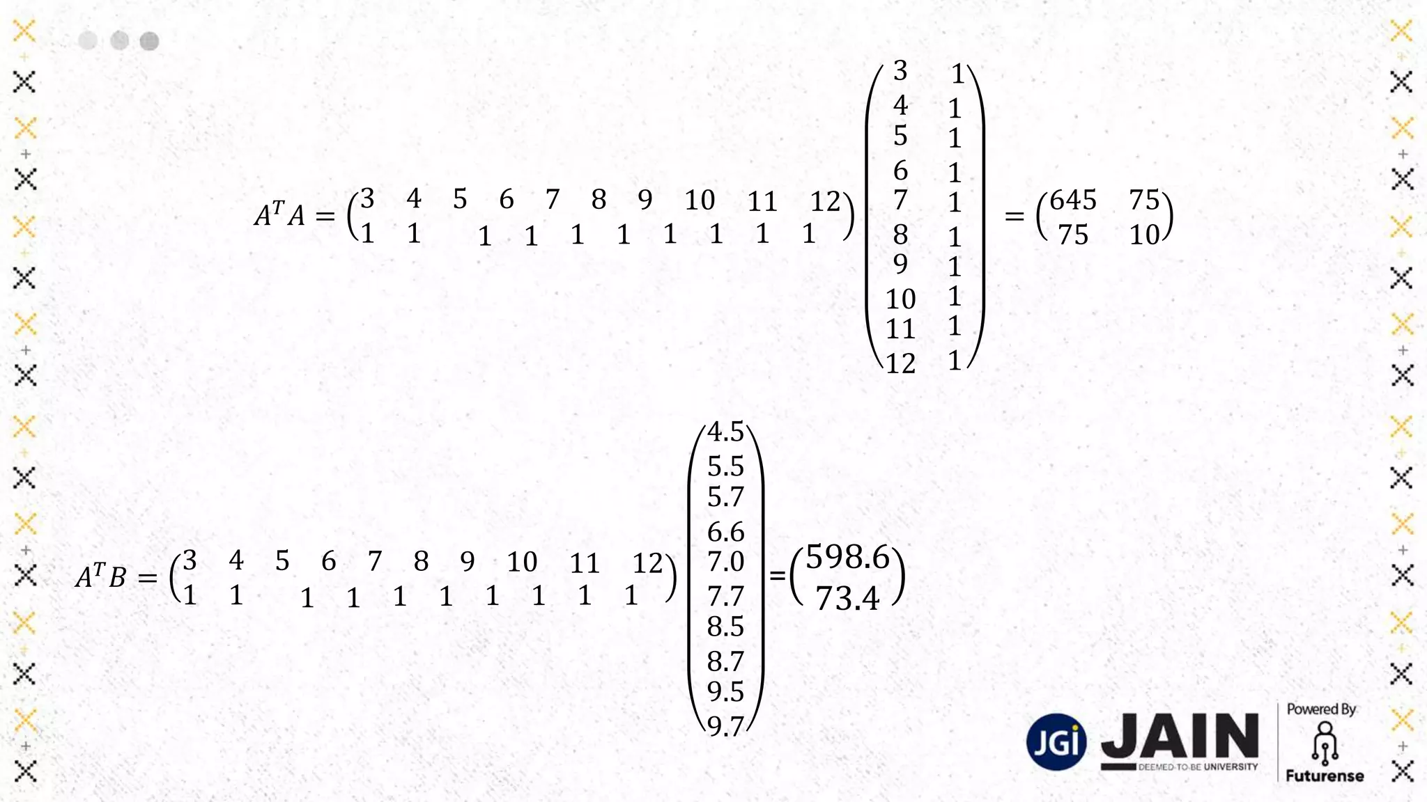
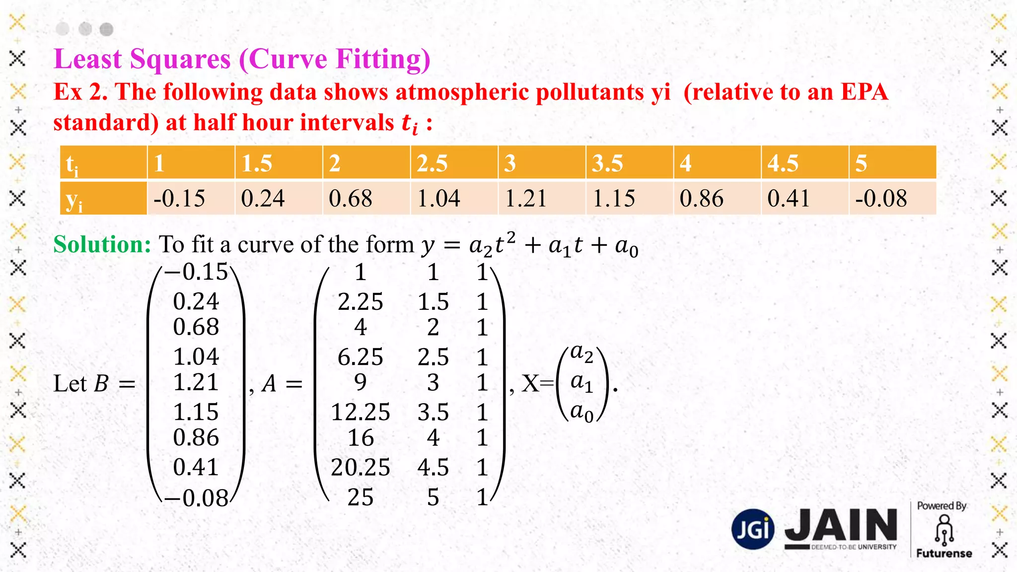
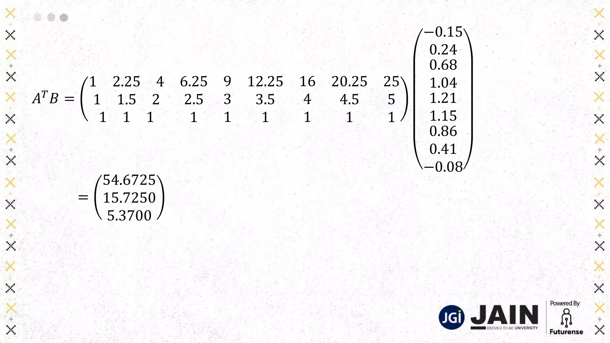
This document discusses various matrix decomposition techniques including least squares, eigendecomposition, and singular value decomposition. It begins with an introduction to the importance of linear algebra and decompositions for applications. Then it provides examples of using least squares to fit curves to data and find regression lines. It defines eigenvalues and eigenvectors and provides examples of eigendecomposition. It also discusses diagonalization of matrices and using the eigendecomposition to raise matrices to powers. Finally, it discusses singular value decomposition and its applications.

1. Probability and Vector Spaces

2. MODULE 5:
Department of Mathematics
Jain Global campus, Jakkasandra Post, Kanakapura Taluk, Ramanagara District -562112
Department of Mathematics
FET-JAIN (Deemed-to-be University)
Matrix Decomposition

3. Table of Content
• Aim
• Introduction
• Objective
• Curve Fitting-Least Squares
• Eigen Values and Eigen Vectors
• Eigen Value Decomposition
• Singular Value Decomposition
• Reference Links

4. Aim
To equip students in the fundamental concepts of decomposition of matrices so
that they can simplify more complex matrix operations that can be performed on
the decomposed matrix rather than on the original matrix itself, which is helpful
in simplifying data, removing noise, may improving algorithm results

5. Objective
a. Discuss the Least square method for curve fitting.
b. Define Eigen values and Eigen vectors of a matrix
c. Describe the examples of Eigen value decomposition
d. Discuss the singular value decomposition method
e. Describe the examples of singular value decomposition

6. Introduction
The importance of linear algebra for applications has risen in direct proportion to
the increase in computing power, with each new generation of hardware and software
triggering a demand for even greater capabilities. Computer science is thus intricately
linked with linear algebra through the explosive growth of parallel processing and large-
scale computations.

7. Least Squares (Curve Fitting)
Working rule: Quadratic fit
Curve: 𝒚 = 𝒂𝟐𝒙𝟐 + 𝒂𝟏𝒙 + 𝒂𝟎
Step 1. Form 𝐵 =
𝑦1
𝑦2
⋮
𝑦𝑛
, 𝐴 =
𝑥1
2
𝑥1 1
𝑥2
2 𝑥2 1
⋮
𝑥𝑛
2
⋮
𝑥𝑛
⋮
1
and 𝑋 =
𝑎2
𝑎1
𝑎0
.
Step 2. Solve the normal system: 𝐴𝑇
𝐴𝑋 = 𝐴𝑇
𝐵, for finding X by Gauss Jordan reduction.

8. Least Squares (Curve Fitting)
Working rule: Linear Fit
Curve: 𝒚 = 𝒂𝟏𝒙 + 𝒂𝟎
Step 1. Form 𝐵 =
𝑦1
𝑦2
⋮
𝑦𝑛
, 𝐴 =
𝑥1 1
𝑥2 1
⋮
𝑥𝑛
⋮
1
, 𝑋 =
𝑎1
𝑎0
Step 2. Solve the normal system: 𝐴𝑇
𝐴𝑋 = 𝐴𝑇
𝐵, for finding X by Gauss Jordan
reduction.

9. Least Squares (Curve Fitting)
Ex 1. In the manufacturing of product X, the amount of the compound beta present
in the product is controlled by the amount of independent alpha used in the process.
In manufacturing a gallon of X, the amount of alpha used and the amount of beta
present are recorded. The following data were obtained:
Find an equation of the least square line for the data.
Use the equation obtained to predict the number of gallons beta present in a gallon
of product X, if 30 gallons of alpha are used per gallon.
Alpha used (x)
(gallon)
3 4 5 6 7 8 9 10 11 12
Beta present (y)
(gallon)
4.5 5.5 5.7 6.6 7.0 7.7 8.5 8.7 9.5 9.7

10. Solution:
To fit a curve of the form 𝑦 = 𝑎1𝑥 + 𝑎0
𝐵 =
4.5
5.5
5.7
6.6
7.0
7.7
8.5
8.7
9.5
9.7
, 𝐴 =
3
4
5
6
7
8
9
10
11
12
1
1
1
1
1
1
1
1
1
1
, 𝑋 =
𝑎1
𝑎0
.

11. 𝐴𝑇𝐴 =
3 4 5 6 7 8 9 10 11 12
1 1 1 1 1 1 1 1 1 1
3
4
5
6
7
8
9
10
11
12
1
1
1
1
1
1
1
1
1
1
=
645 75
75 10
𝐴𝑇𝐵 =
3 4 5 6 7 8 9 10 11 12
1 1 1 1 1 1 1 1 1 1
4.5
5.5
5.7
6.6
7.0
7.7
8.5
8.7
9.5
9.7
=
598.6
73.4

12. 𝐴𝑇
𝐴𝑋 = 𝐴𝑇
𝐵
645 75
75 10
𝑎1
𝑎0
=
598.6
73.4
𝑎1
𝑎0
=
645 75
75 10
−1
.
598.6
73.4
=
0.0121 −0.09
−0.09 0.7818
.
598.6
73.4
=
0.5830
2.9672
𝑌 = 0.5830 𝑥 + 2.9672
𝑌𝑥=30 = 0.5830 30 + 2.9672 = 20.4572

13. Least Squares (Curve Fitting)
Ex 2. The following data shows atmospheric pollutants yi (relative to an EPA
standard) at half hour intervals 𝒕𝒊 :
Solution: To fit a curve of the form 𝑦 = 𝑎2𝑡2 + 𝑎1𝑡 + 𝑎0
Let 𝐵 =
−0.15
0.24
0.68
1.04
1.21
1.15
0.86
0.41
−0.08
, 𝐴 =
1 1 1
2.25 1.5 1
4
6.25
9
12.25
16
20.25
25
2
2.5
3
3.5
4
4.5
5
1
1
1
1
1
1
1
, X=
𝑎2
𝑎1
𝑎0
.
ti 1 1.5 2 2.5 3 3.5 4 4.5 5
yi -0.15 0.24 0.68 1.04 1.21 1.15 0.86 0.41 -0.08

14. 𝐴𝑇𝐵 =
1 2.25 4
1 1.5 2
1 1 1
6.25
2.5
1
9
3
1
12.25
3.5
1
16
4
1
20.25
4.5
1
25
5
1
−0.15
0.24
0.68
1.04
1.21
1.15
0.86
0.41
−0.08
=
54.6725
15.7250
5.3700

15. Solve 𝐴𝑇
𝐴𝑋 = 𝐴𝑇
𝐵
𝑋 = (𝐴𝑇
𝐴)−1
. 𝐴𝑇
𝐵
=
1583.25 378 96
378 96 27
96 27 9
−1
.
54.6725
15.7250
5.3700
=
0.0519 −0.311 0.3809
−0.311 1.9367 −2.485
0.3809 −2.485 3.5047
.
54.6725
15.7250
5.3700
=
−0.32714
2.0038
−1.9250
𝑦 = −0.32714 𝑡2
+ 2.0038 𝑡 + (−1.9250)

16. Questions for practice
1. The distributor of new car has obtained the following data
Number of weeks after
introduction a car
1 2 3 4 5 6 7 8 9 10
Gross Receipts per
week(millions of dollars)
0.8 0.5 3.2 4.3 4 5.1 4.3 3.8 1.2 0.8
t
Let x denote the gross receipts per week (in millions of dollars) t weeks after the
introduction of the car. Use the equation to
a. Find a least squares quadratic polynomial for the given data
b. estimate the gross receipts 12 weeks after the introduction of the car.

17. Questions for practice
2. A steel producer gathers the following data
t
Represent the years 1997-2002 as 0,1,2,3,4,5 respectively. Let x denote the
the year and y denote the annual sales. Then
a. Find the least square line relating to x and y
b. Use the obtained equation to estimate the annual sale in 2006.
Year 1997 1998 1999 2000 2001 2002
Annual Sales
(Millions of
dollars)
1.2 2.3 3.2 3.6 3.8 5.1

18. Eigenvalues and Eigenvectors
Definition:
An eigenvector of an 𝑛 × 𝑛 matrix A is a nonzero vector x such that 𝐴𝑥 = λx for some
scalar λ. A scalar λ is called an eigenvalue of A if there is a nontrivial solution x of 𝐴𝑥 =
λx. Such an x is called an eigenvector corresponding to λ.
Definition:
Let A be the matrix then 𝑑𝑒𝑡 𝐴 − λI = 0 is called the characteristic equation A.
Note:
i) Here row reduction concept was used to find the eigenvector, it cannot be used to find
eigenvalues.
ii) An echelon form of a matrix A usually does not display the eigenvalues of A.
iii) Thus, 𝝺 is an eigenvalue of A if and only if the equation 𝑨 − 𝞴𝑰 𝒙 = 𝟎 →∗ has a
nontrivial solution.

19. Example 1: Let 𝐴 =
1 6
5 2
𝑢 =
6
−5
and 𝑣 =
3
−2
. Are u and v eigenvectors of A?
Solution:
𝐴𝑢 =
1 6
5 2
6
−5
=
6 − 30
30 − 10
=
−24
20
= −4
6
−5
= −4𝑢
𝐴𝑣 =
1 6
5 2
3
−2
=
−9
11
≠ λ
3
−2
.
Thus, u is an eigenvector corresponding to an eigenvalue -4, but v is not an eigenvector of A, because Av is not a
multiple of v.

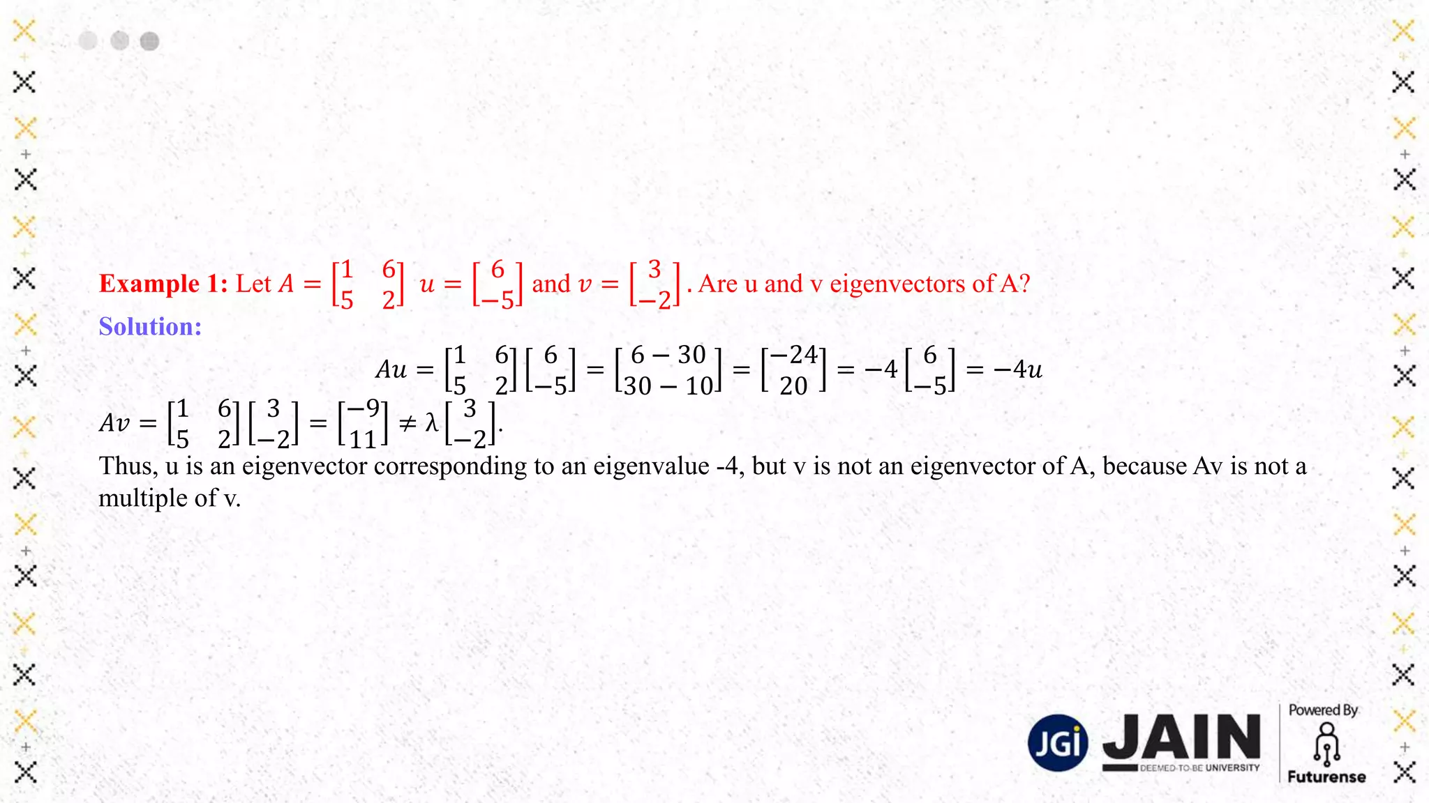
20. Example 2: Show that 7 is an eigenvalue of the matrix 𝑨 =
𝟏 𝟔
𝟓 𝟐
and find the
corresponding eigenvectors.
Solution:
The scalar 7 is an eigenvalue of A iff the equation 𝐴𝑥 = 7𝑥 has a nontrivial solution, i.e.
𝐴𝑥 − 7𝑥 = 0 𝑜𝑟 𝐴 − 7𝐼 𝑥 = 0 → (1)
To solve this homogeneous equation, form the matrix 𝐴 − 7𝐼 =
−6 6
5 −5
.
The columns of 𝐴 − 7𝐼 are obviously linear dependent (multiple of each other). So
equation(1) has nontrivial solution. Thus 7 is an Eigen value of A.
To find the corresponding eigenvectors use row operations
Which implies[A:B]=
−6 6:
5 −5:
0
0
𝑅1 → −
1
6
𝑅1 𝑎𝑛𝑑 𝑅2 →
1
5
𝑅2
Then
1 −1:
0 0:
0
0
which gives 𝑥1 = 𝑥2, the general solution 𝑋 =
𝑥1
𝑥2
=
𝑥2
𝑥2
=
1
1
.
Each vector of this form with 𝑥2 ≠ 0 is an eigenvector corresponding 𝜆 = 7.

21. Diagonalization of Matrix
The diagonalization Theorem: An 𝑛 × 𝑛 matrix A is diagonalizable if and only if A has
n linearly independent eigenvectors.
In fact 𝐴 = 𝑃𝐷𝑃−1, with D is a diagonal matrix, iff the columns of P are n linearly
independent eigenvectors of A. In this case the diagonal entries of D are eigenvalues of
A corresponding to eigenvectors in P.
Theorem: An 𝑛 × 𝑛 matrix with n distinct eigenvalues is diagonalizable.
Modal Matrix:
Consider a square matrix of order 3 × 3, Let λ1, λ2, λ3 be the Eigen values and the
corresponding eigenvectors 𝑋1, 𝑋2, 𝑋3 then 𝑃 = (𝑋1, 𝑋2, 𝑋3) is called as modal matrix
and 𝐷 =
𝜆1 0 0
0 𝜆2 0
0 0 𝜆3
is called a diagonal matrix.

22. Power of Matrix A:
Consider 𝐷2
= 𝐷. 𝐷
𝐷2
= (𝑃−1
𝐴𝑃)(𝑃−1
𝐴𝑃)
= 𝑃−1𝐴𝑃𝑃−1𝐴𝑃
=𝑃−1 𝐴𝐼𝐴 𝑃
=𝑃−1𝐴𝐴𝑃
𝐷2 = 𝑃−1𝐴2𝑃
𝑃𝐷2𝑃−1 = 𝑃𝑃−1𝐴2𝑃𝑃−1
𝑃𝐷2𝑃−1 = 𝐴2
Which implies 𝐴𝑛 = 𝑃𝐷𝑛𝑃−1 where 𝐷𝑛 =
𝜆1
𝑛
0 0
0 𝜆2
𝑛
0
0 0 𝜆3
𝑛

23. Eigenvalue Decomposition: Or Orthogonal diagonalization
Definition:
A matrix is said to be orthogonally diagonalizable if there are an orthogonal matrix P
(with 𝑃−1
= 𝑃𝑇
) and a diagonal matrix D such that 𝐴 = 𝑃𝐷𝑃−1
=𝑃𝐷𝑃𝑇
.
Theorem:
An 𝑚 × 𝑛 matrix A is orthogonally diagonalizable iff A is a symmetric Matrix
Note:
1. An orthogonal matrix is a square matrix with orthonormal columns.
2. A n orthogonally diagonalizable matrix is a special kind of diagonalizable
matrix: not only can we factor 𝐴 = 𝑃𝐷𝑃−1 , but we can find an orthonormal
columns.
3. A set of vectors S is orthonormal if every vector in S has magnitude 1 and the set of

24. Example1: If possible, orthogonally diagonalize the matrix 𝐴 =
6 −2 −1
−2 6 −1
−1 −1 5
Solution:
The characteristic equation is 𝐴 − 𝜆𝐼 = 0 implies
6 −2 −1
−2 6 −1
−1 −1 5
= 0
Which implies 𝜆3 − 11𝜆2 + 90𝜆 − 144 = 0, the Eigen values are 𝜆 = 8,6,3
For 𝜆 = 8, we have 𝐴 − 8𝐼, 0 =
−2 −2 −1
−2 −2 −1
−1 −1 −3
0
0
0
after row transformation we get
1 1 0
0 0 1
0 0 0
0
0
0
which implies 𝑥1 + 𝑥2 = 0 → 𝑋 =
𝑥1
𝑥2
𝑥3
=
−𝑥2
𝑥2
0
= 𝑥2
−1
1
0
, then
𝑣1 =
−1
1
0
.

25. Let 𝜆 = 6, we have 𝐴 − 6𝐼, 0 =
0 −2 −1
−2 0 −1
−1 −1 −1
0
0
0
after row transformation we get
Then
1 −1 0
0 −2 −1
0 0 0
0
0
0
implies 𝑋 =
𝑥1
𝑥2
𝑥3
= 𝑥3
−1
−1
2
, thus the 𝑣2 =
−1
−1
2
.
And for 𝜆 = 3, we have 𝐴 − 3𝐼, 0 =
3 −2 −1
−2 3 −1
−1 −1 2
0
0
0
after row transformation
we get
−1 1 0
0 1 −1
0 0 0
0
0
0
implies 𝑋 =
𝑥1
𝑥2
𝑥3
= 𝑥3
1
1
1
, thus the 𝑣3 =
1
1
1
.
Clearly these 𝑣1, 𝑣2, 𝑣3 vectors are basis for 𝑅3.

26. Since a nonzero multiple of an eigenvector is still an eigenvector. We can normalize
𝑣1, 𝑣2, 𝑣3 to produce the unit eigenvectors.
Then 𝑢1 =
𝑣1
𝑣1
=
−
1
2
1
2
0
, 𝑢2 =
𝑣2
𝑣2
=
−
1
6
−
1
6
2
6
and 𝑢3 =
𝑣3
𝑣3
=
1
3
1
3
1
3
.
Let 𝑃 =
−
1
2
1
2
0
−
1
6
−
1
6
2
6
1
3
1
3
1
3
and 𝐷 =
8 0 0
0 6 0
0 0 3
.
Then 𝐴 = 𝑃𝐷𝑃−1 as usual. But this time P is square matrix and has orthonormal
columns, P is orthogonal matrix and 𝑃−1 is simply 𝑃𝑇.

27. Questions for practice
1. Orthogonally diagonalize the matrix 𝑨 =
𝟑 −𝟐 𝟒
−𝟐 𝟔 𝟐
𝟒 𝟐 𝟑
whose characteristic
equation is −𝝀𝟑
+ 𝟏𝟐𝝀𝟐
− 𝟐𝟏𝝀 − 𝟗𝟖 = 𝟎 = − 𝝀 − 𝟕 𝟐
(𝝀 + 𝟐).
2. Orthogonally diagonalize the matrix 𝑨 =
𝟏 𝟔 𝟏
𝟏 𝟐 𝟎
𝟎 𝟎 𝟑

28. Singular Value Decomposition
Singular values:
The square root of eigen values of a symmetric matrix ATA or AAT are called singular
values of the matrix A.
Singular Vectors:
The eigen vectors of ATA corresponding to singular values of A are called singular
vectors.
The singular vectors of ATA are called right singular vectors and singular vectors of AAT
are called left singular vectors.
Definition of SVD:
Let A be any matrix m × n then this matrix can be decomposed in to product of three
matrices given by Am×n =Um×m Σm×nVT
n×n and it is called singular value decomposition of
A.
Where U and V are called orthogonal matrices or unitary matrices and Σ is called
singular matrix.

29. Important points on SVD:
The SVD produces orthonormal bases of v’s and u’ for the four fundamental subspaces.
Using those bases, A becomes a diagonal matrix Σ and Avi = σiui and σi = singular value.
The two-bases diagonalization A = UΣVT often has more information than A = PDP−1
UΣVT separates A into rank-1 matrices
σ1u1vT
1 + σ2u2vT
2 + ........ + σrurvT
r . σ1u1v T 1 is the largest.
u1,u2 ,..., ur is an orthonormal basis for the column space
ur+1, ur+2 ...,um is an orthonormal basis for left null space N (AT)
v1,v2 ..., vr is an orthonormal basis for the row space
vr+1,vr+2 ..., vn is an orthonormal basis for the null space N(A).

30. Working Rule
Step-1: Compute ATA or AAT.
Step-2: Find the eigen values of ATA or AAT.
Step-3: Compute the square root of non-zero eigen values of above step called singular
values of A.
Step-4: Construct a singular matrix Σ of order same as A having singular values on the
diagonal in decreasing order.
Step-5: Find the eigen vector of ATA or AAT and construct a orthogonal matrix V or U
consisting of orthonormal eigen vectors of ATA or AAT.
Step-6: Construct the vectors ui = Aviσi or vi =ATui σi and the orthogonal matrix U or V
respectively.
Step-7: Finally, A = UΣVT gives the singular value decomposition of matrix A

31. Example: Find Singular value decomposition of the matrix 𝑨 =
−𝟑 𝟏
𝟔 −𝟐
𝟔 −𝟐
Solution:

37. Hence the orthogonal matrix 𝑈 = 𝑢1, 𝑢2, 𝑢3 or matrix of left singular vectors is
given by

38. Questions for practice
1. Find Singular value decomposition of the matrix 𝑨 =
𝟏 𝟏 𝟏
𝟏 𝟏 𝟏
2. Find Singular value decomposition of the matrix 𝑨 =
𝟏 −𝟏
−𝟐 𝟐
𝟐 −𝟐
.

39. Summary
Outcomes:
a. Discuss the concept of curve fitting using least square sense and its application in
engineering.
b. Describe the importance of diagonalization to tackle engineering problems.