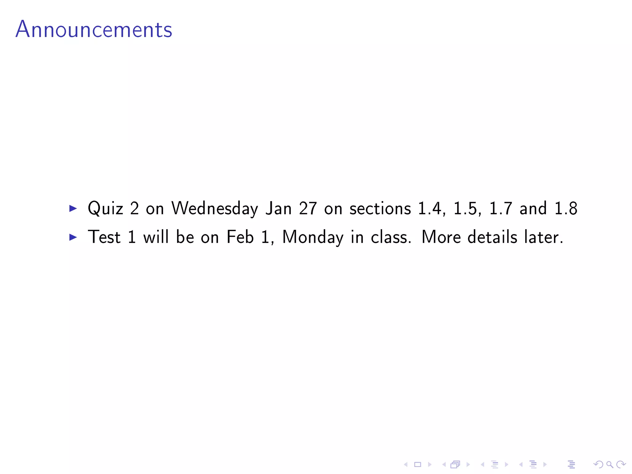
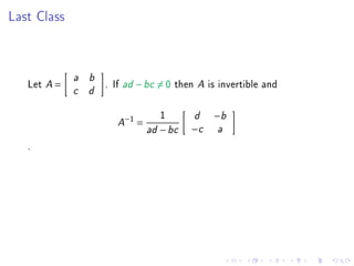
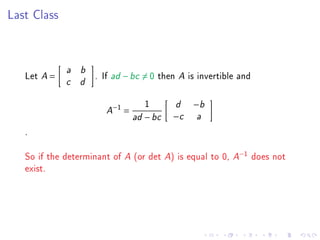
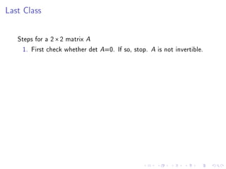
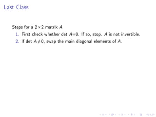
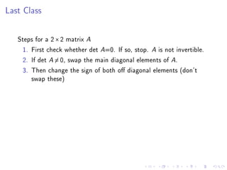
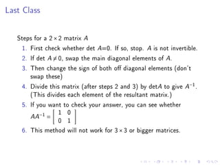
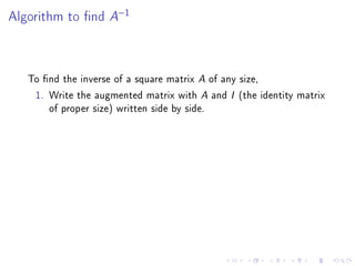
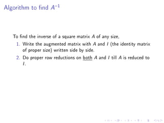
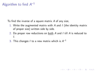
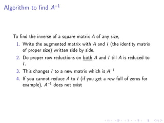
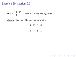
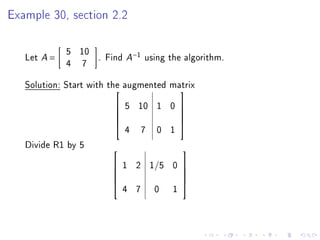
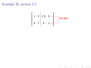
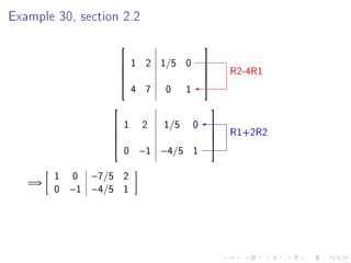
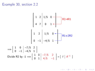
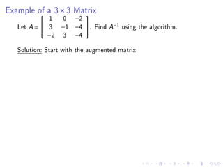
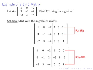
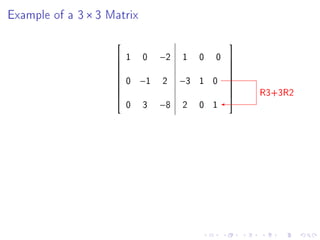
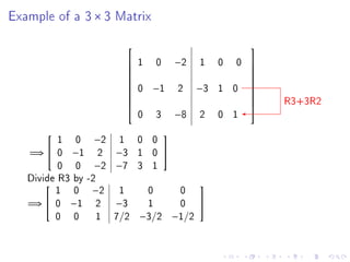
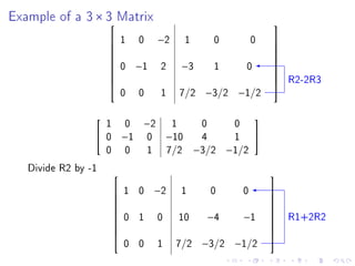
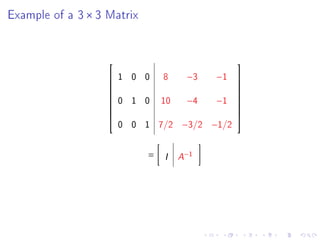
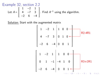
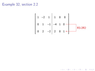
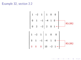
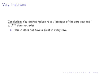
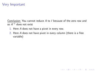
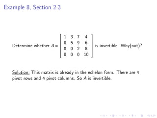
Announcements


     Quiz 2 on Wednesday Jan 27 on sections 1.4, 1.5, 1.7 and 1.8
     Test 1 will be on Feb 1, Monday in class. More details later.
Last Class


             a   b
   Let A =           . If ad − bc = 0 then A is invertible and
             c   d


                           −1          1      d    −b
                       A        =
                                    ad − bc   −c   a

   .
Last Class


             a   b
   Let A =           . If ad − bc = 0 then A is invertible and
             c   d


                           −1          1      d    −b
                       A        =
                                    ad − bc   −c   a

   .

   So if the determinant of A (or det A) is equal to 0, A−1 does not
   exist.
Last Class


   Steps for a 2 × 2 matrix A
    1. First check whether det A=0. If so, stop.   A   is not invertible.
Last Class


   Steps for a 2 × 2 matrix A
    1. First check whether det A=0. If so, stop. A is not invertible.
    2. If det A = 0, swap the main diagonal elements of A.
Last Class


   Steps for a 2 × 2 matrix A
    1. First check whether det A=0. If so, stop. A is not invertible.
    2. If det A = 0, swap the main diagonal elements of A.
    3. Then change the sign of both o diagonal elements (don't
       swap these)
Last Class


   Steps for a 2 × 2 matrix A
    1. First check whether det A=0. If so, stop. A is not invertible.
    2. If det A = 0, swap the main diagonal elements of A.
    3. Then change the sign of both o diagonal elements (don't
       swap these)
    4. Divide this matrix (after steps 2 and 3) by detA to give A−1 .
       (This divides each element of the resultant matrix.)
    5. If you want to check your answer, you can see whether
                   1 0
       AA−1 =
                   0 1
    6. This method will not work for 3 × 3 or bigger matrices.
Example 7(a) section 2.2, One Case
            1 2
   Let A =          . Find A−1 and use it to solve the equation
            5 12
                        2
   Ax = b3 where b3 =
                        6

   Solution: Here detA = (1)(12) − (5)(2) = 2 = 0. So we can nd A−1 .
Example 7(a) section 2.2, One Case
            1 2
   Let A =          . Find A−1 and use it to solve the equation
            5 12
                        2
   Ax = b3 where b3 =
                        6

   Solution: Here detA = (1)(12) − (5)(2) = 2 = 0. So we can nd A−1 .
   Interchange the positions of 1 and 12. Change the signs of 2 and 5.
   Then we get
                                  12 −2
                                 −5 1
   .
Example 7(a) section 2.2, One Case
            1 2
   Let A =          . Find A−1 and use it to solve the equation
            5 12
                        2
   Ax = b3 where b3 =
                        6

   Solution: Here detA = (1)(12) − (5)(2) = 2 = 0. So we can nd A−1 .
   Interchange the positions of 1 and 12. Change the signs of 2 and 5.
   Then we get
                                  12 −2
                                 −5 1
   . Divide each element of the matrix by detA which is 2. This gives
                           −1        6     −1
                          A =
                                   −5/2 1/2

                    x1         6         −1     2       6
              x=         =                          =
                    x2       −5/2        1 /2   6       −2
                                   A−1          b
Algorithm to nd    A−1


   To nd the inverse of a square matrix A of any size,
    1. Write the augmented matrix with A and I (the identity matrix
       of proper size) written side by side.
Algorithm to nd    A−1


   To nd the inverse of a square matrix A of any size,
    1. Write the augmented matrix with A and I (the identity matrix
       of proper size) written side by side.
    2. Do proper row reductions on both A and I till A is reduced to
       I.
Algorithm to nd    A−1


   To nd the inverse of a square matrix A of any size,
    1. Write the augmented matrix with A and I (the identity matrix
       of proper size) written side by side.
    2. Do proper row reductions on both A and I till A is reduced to
       I.
    3. This changes I to a new matrix which is A−1
Algorithm to nd     A−1


   To nd the inverse of a square matrix A of any size,
    1. Write the augmented matrix with A and I (the identity matrix
       of proper size) written side by side.
    2. Do proper row reductions on both A and I till A is reduced to
       I.
    3. This changes I to a new matrix which is A−1
    4. If you cannot reduce A to I (if you get a row full of zeros for
       example), A−1 does not exist
Example 30, section 2.2

             5 10
   Let A =        . Find A−1 using the algorithm.
             4 7
   Solution: Start with the augmented matrix
                                       
                        
                        
                            5 10 1 0      
                                          
                                         
                            4   7   0 1
                                         
Example 30, section 2.2

             5 10
   Let A =        . Find A−1 using the algorithm.
             4 7
   Solution: Start with the augmented matrix
                                       
                        
                        
                            5 10 1 0          
                                              
                                             
                            4     7   0 1
                                             

   Divide R1 by 5                            
                        
                        
                            1 2 1/5 0         
                                              
                                             
                            4 7       0   1
                                             
Example 30, section 2.2
                                    
                       1 2 1/5 0
                                         R2-4R1
                                    
                                    
                                    
                       4 7   0   1
                                    
Example 30, section 2.2
                                             
                          1 2 1/5 0
                                                      R2-4R1
                                             
                                             
                                             
                          4 7   0     1
                                             

                                                 
                      1    2    1/5       0
                                                      R1+2R2
                                                 
                                                 
                                                 
                      0    −1 −4/5        1
                                                 


        1   0 −7/5    2
   =⇒
        0   −1 −4/5   1
Example 30, section 2.2
                                                
                            1 2 1/5 0
                                                         R2-4R1
                                                
                                                
                                                
                            4 7    0     1
                                                

                                                    
                        1    2     1/5       0
                                                         R1+2R2
                                                    
                                                    
                                                    
                        0    −1 −4/5         1
                                                    


        1   0 −7/5      2
   =⇒
        0   −1 −4/5     1
                         1 0      −7/5       2
   Divide R2 by -1 =⇒                                =   I   A−1
                         0 1      4/5    −1
Example of a 3 × 3 Matrix
             1    0 −2
                    

   Let A =  3    −1 −4 .   Find A−1 using the algorithm.
             −2   3 −4
   Solution: Start with the augmented matrix
Example of a 3 × 3 Matrix
             1    0 −2
                    

   Let A =  3    −1 −4 .       Find A−1 using the algorithm.
             −2   3 −4
   Solution: Start with the augmented matrix
                                                         
                            1      0   −2   1 0 0        
                                                                 R2-3R1
                                                         
                                                         
                             3     −1 −4     0 1 0
                                                         
                                                         
                                                         
                                                         
                            −2      3   −4   0 0      1
                                                         


                                                         
                           1      0    −2   1    0 0     
                                                         
                                                         
                            0     −1    2    −3   1   0          R3+2R1
                                                         
                                                         
                                                         
                                                         
                            −2     3    −4   0    0 1
                                                         
Example of a 3 × 3 Matrix

                                                  
                       1   0    −2   1    0   0   
                                                  
                                                  
                        0   −1   2    −3   1 0
                                                  
                                                  
                                                       R3+3R2
                                                  
                                                  
                        0   3    −8   2    0 1
                                                  
Example of a 3 × 3 Matrix

                                                     
                       1   0       −2   1    0   0   
                                                     
                                                     
                        0   −1      2    −3   1 0
                                                     
                                                     
                                                          R3+3R2
                                                     
                                                     
                        0   3       −8   2    0 1
                                                     


          1 0 −2 1 0 0
                               

   =⇒  0 −1 2 −3 1 0 
          0 0 −2 −7 3 1
   Divide R3 by -2
         1 0 −2 1     0  0
                                        

   =⇒  0 −1 2     −3 1  0               
         0 0 1 7/2 −3/2 −1/2
Example of a 3 × 3 Matrix
                                                                          
                            1    0       −2         1      0          0   
                                                                          
                                                                          
                             0    −1       2     −3         1      0
                                                                          
                                                                          
                                                                               R2-2R3
                                                                          
                                                                          
                             0    0        1     7 /2      −3/2 −1/2
                                                                          


                     1       0     −2           1         0      0
                                                                      
                    0       −1       0       −10         4      1     
                     0       0        1       7 /2       −3/2   −1/2
   Divide R2 by -1                                                        
                            1 0          −2     1          0      0       
                                                                          
                                                                          
                             0 1          0     10         −4      −1          R1+2R2
                                                                          
                                                                          
                                                                          
                                                                          
                             0 0          1     7/2       −3/2 −1/2
                                                                          
Example of a 3 × 3 Matrix


                                                
                      1 0 0    8     −3   −1    
                                                
                                                
                       0 1 0    10    −4   −1
                                                
                                                
                                                
                                                
                       0 0 1 7 /2    −3/2 −1/2
                                                


                            =   I    A−1
Example 32, section 2.2
             1    −2   1
                     

   Let A =  4    −7   3 . Find A−1 using the algorithm.
             −2   6    −4

   Solution: Start with the augmented matrix
                                                      
                            1   −2    1   1 0 0       
                                                            R2-4R1
                                                      
                                                      
                             4   −7    3   0 1 0
                                                      
                                                      
                                                      
                                                      
                            −2    6   −4   0 0     1
                                                      


                                                      
                           1    −2   1    1   0 0     
                                                      
                                                      
                            0    1    −1 −4    1   0        R3+2R1
                                                      
                                                      
                                                      
                                                      
                            −2   6    −4   0   0 1
                                                      
Example 32, section 2.2

                                                 
                       1   −2   1    1   0   0   
                                                 
                                                 
                        0   1    −1 −4    1 0
                                                 
                                                 
                                                      R3-2R2
                                                 
                                                 
                        0   2    −2   2   0 1
                                                 
Example 32, section 2.2

                                                    
                       1   −2    1    1   0    0    
                                                    
                                                    
                        0    1   −1 −4     1 0
                                                    
                                                    
                                                         R3-2R2
                                                    
                                                    
                        0    2   −2    2   0 1
                                                    


                                                    
                       1   −2   1    1    0     0   
                                                    
                                                    
                        0   1    −1 −4     1    0
                                                    
                                                    
                                                         R3-2R2
                                                    
                                                    
                        0   0    0    10   −2   1
                                                    
Very Important


   Conclusion: You cannot reduce A to I because of the zero row and
   so A−1 does not exist
     1. Here A does not have a pivot in every row.
Very Important


   Conclusion: You cannot reduce A to I because of the zero row and
   so A−1 does not exist
     1. Here A does not have a pivot in every row.
     2. Here A does not have pivot in every column (there is a free
        variable)
Very Important


   Conclusion: You cannot reduce A to I because of the zero row and
   so A−1 does not exist
     1. Here A does not have a pivot in every row.
     2. Here A does not have pivot in every column (there is a free
        variable)
     3. The equation Ax = 0 has Non-trivial solution
Very Important


   Conclusion: You cannot reduce A to I because of the zero row and
   so A−1 does not exist
     1. Here A does not have a pivot in every row.
     2. Here A does not have pivot in every column (there is a free
        variable)
     3. The equation Ax = 0 has Non-trivial solution
     4. The columns of A are linearly
Very Important


   Conclusion: You cannot reduce A to I because of the zero row and
   so A−1 does not exist
     1. Here A does not have a pivot in every row.
     2. Here A does not have pivot in every column (there is a free
        variable)
     3. The equation Ax = 0 has Non-trivial solution
     4. The columns of A are linearly Dependent
     5. A cannot be row-reduced to the 3 × 3 identity matrix
Section 2.3 Invertible Matrices

   If a square matrix A of size n × n is invertible the following is true
Section 2.3 Invertible Matrices

   If a square matrix A of size n × n is invertible the following is true
   Theorem
   The Invertible Matrix Theorem (IMT)

    1.   A has n pivot positions (n pivot rows and n pivot columns)
Section 2.3 Invertible Matrices

   If a square matrix A of size n × n is invertible the following is true
   Theorem
   The Invertible Matrix Theorem (IMT)

    1.   A has n pivot positions (n pivot rows and n pivot columns)
    2.   A can be row-reduced to the n × n identity matrix
Section 2.3 Invertible Matrices

   If a square matrix A of size n × n is invertible the following is true
   Theorem
   The Invertible Matrix Theorem (IMT)

    1.   A has n pivot positions (n pivot rows and n pivot columns)
    2.   A can be row-reduced to the n × n identity matrix
    3.   The equation Ax = 0 has only the trivial solution (no free
         variables)
    4.   The columns of A are linearly
Section 2.3 Invertible Matrices

   If a square matrix A of size n × n is invertible the following is true
   Theorem
   The Invertible Matrix Theorem (IMT)

    1.   A has n pivot positions (n pivot rows and n pivot columns)
    2.   A can be row-reduced to the n × n identity matrix
    3.   The equation Ax = 0 has only the trivial solution (no free
         variables)
    4.   The columns of A are linearly independent
    5.   The equation Ax = b is consistent for every   b   in Rn
    6.   The columns of A span Rn (because every row has a pivot and
         recall theorem 4, sec 1.4)
Example 2, Section 2.3


                           −4   6
   Determine whether A =             is invertible. Why(not)?
                           6    −9
Example 2, Section 2.3


                              −4   6
   Determine whether A =                 is invertible. Why(not)?
                               6   −9

   Solution: Clearly the determinant is (-4)(-9)-(6)(6)=36-36=0. So
   not invertible. Checking invertibility of 2 × 2 matrices are thus easy.
   Not so obvious fact: The second column is -1.5 times the rst
   column. Since we have linearly dependent columns, by IMT, A is
   not invertible.
Example 4, Section 2.3


                              −7   0    4
                                           

   Determine whether A =  3       0   −1      is invertible. Why(not)?
                           2       0    9
   Solution: Remember what happens to a set of vectors if the zero
   vector is present in that set?
Example 4, Section 2.3


                               −7   0    4
                                            

   Determine whether A =  3        0   −1      is invertible. Why(not)?
                           2        0    9
   Solution: Remember what happens to a set of vectors if the zero
   vector is present in that set? The vectors are linearly dependent.


   Since the second column of A is full of zeros, we have linearly
   dependent columns, and so A is not invertible.
Example 6, Section 2.3
                              1        −5 −4
                                                      

   Determine whether A =     0        3           4      is invertible. Why(not)?
                              −3       6           0
                                                      
                         1    −5 −4                   
                                                      
                                                      
                          0        3           4              R3+3R1
                                                      
                                                      
                                                      
                                                      
                          −3       6       0
                                                      


                                                      
                         1    −5          −4          
                                                      
                                                      
                          0    3           4
                                                      
                                                      
                                                              R3+3R2
                                                      
                                                      
                          0    −9 −12
                                                      
Example 6, Section 2.3


                                    
                        1   −5 −4 
                                  
                                  
                         0   3 4 
                                  
                    
                                  
                                  
                         0   0   0
                                  
Example 6, Section 2.3


                                        
                            1   −5 −4 
                                      
                                      
                             0   3 4 
                                      
                         
                                      
                                      
                             0   0   0
                                      


   Since the third row (and the third column) does not have a pivot,
   we have linearly dependent columns and by the IMT A is not
   invertible.
Example 8, Section 2.3


                             1   3   7 4
                                           
                            0   5   9 6    
   Determine whether A =                   
                                                is invertible. Why(not)?
                             0   0   2 8
                                           
                                           
                             0   0   0 10
Example 8, Section 2.3


                              1   3   7 4
                                            
                             0   5   9 6    
   Determine whether A =                    
                                                 is invertible. Why(not)?
                              0   0   2 8
                                            
                                            
                              0   0   0 10


   Solution: This matrix is already in the echelon form. There are 4
   pivot rows and 4 pivot columns. So A is invertible.

Matrix Inverse, IMT

  • 1.
    Announcements Quiz 2 on Wednesday Jan 27 on sections 1.4, 1.5, 1.7 and 1.8 Test 1 will be on Feb 1, Monday in class. More details later.
  • 2.
    Last Class a b Let A = . If ad − bc = 0 then A is invertible and c d −1 1 d −b A = ad − bc −c a .
  • 3.
    Last Class a b Let A = . If ad − bc = 0 then A is invertible and c d −1 1 d −b A = ad − bc −c a . So if the determinant of A (or det A) is equal to 0, A−1 does not exist.
  • 4.
    Last Class Steps for a 2 × 2 matrix A 1. First check whether det A=0. If so, stop. A is not invertible.
  • 5.
    Last Class Steps for a 2 × 2 matrix A 1. First check whether det A=0. If so, stop. A is not invertible. 2. If det A = 0, swap the main diagonal elements of A.
  • 6.
    Last Class Steps for a 2 × 2 matrix A 1. First check whether det A=0. If so, stop. A is not invertible. 2. If det A = 0, swap the main diagonal elements of A. 3. Then change the sign of both o diagonal elements (don't swap these)
  • 7.
    Last Class Steps for a 2 × 2 matrix A 1. First check whether det A=0. If so, stop. A is not invertible. 2. If det A = 0, swap the main diagonal elements of A. 3. Then change the sign of both o diagonal elements (don't swap these) 4. Divide this matrix (after steps 2 and 3) by detA to give A−1 . (This divides each element of the resultant matrix.) 5. If you want to check your answer, you can see whether 1 0 AA−1 = 0 1 6. This method will not work for 3 × 3 or bigger matrices.
  • 8.
    Example 7(a) section2.2, One Case 1 2 Let A = . Find A−1 and use it to solve the equation 5 12 2 Ax = b3 where b3 = 6 Solution: Here detA = (1)(12) − (5)(2) = 2 = 0. So we can nd A−1 .
  • 9.
    Example 7(a) section2.2, One Case 1 2 Let A = . Find A−1 and use it to solve the equation 5 12 2 Ax = b3 where b3 = 6 Solution: Here detA = (1)(12) − (5)(2) = 2 = 0. So we can nd A−1 . Interchange the positions of 1 and 12. Change the signs of 2 and 5. Then we get 12 −2 −5 1 .
  • 10.
    Example 7(a) section2.2, One Case 1 2 Let A = . Find A−1 and use it to solve the equation 5 12 2 Ax = b3 where b3 = 6 Solution: Here detA = (1)(12) − (5)(2) = 2 = 0. So we can nd A−1 . Interchange the positions of 1 and 12. Change the signs of 2 and 5. Then we get 12 −2 −5 1 . Divide each element of the matrix by detA which is 2. This gives −1 6 −1 A = −5/2 1/2 x1 6 −1 2 6 x= = = x2 −5/2 1 /2 6 −2 A−1 b
  • 11.
    Algorithm to nd A−1 To nd the inverse of a square matrix A of any size, 1. Write the augmented matrix with A and I (the identity matrix of proper size) written side by side.
  • 12.
    Algorithm to nd A−1 To nd the inverse of a square matrix A of any size, 1. Write the augmented matrix with A and I (the identity matrix of proper size) written side by side. 2. Do proper row reductions on both A and I till A is reduced to I.
  • 13.
    Algorithm to nd A−1 To nd the inverse of a square matrix A of any size, 1. Write the augmented matrix with A and I (the identity matrix of proper size) written side by side. 2. Do proper row reductions on both A and I till A is reduced to I. 3. This changes I to a new matrix which is A−1
  • 14.
    Algorithm to nd A−1 To nd the inverse of a square matrix A of any size, 1. Write the augmented matrix with A and I (the identity matrix of proper size) written side by side. 2. Do proper row reductions on both A and I till A is reduced to I. 3. This changes I to a new matrix which is A−1 4. If you cannot reduce A to I (if you get a row full of zeros for example), A−1 does not exist
  • 15.
    Example 30, section2.2 5 10 Let A = . Find A−1 using the algorithm. 4 7 Solution: Start with the augmented matrix     5 10 1 0     4 7 0 1  
  • 16.
    Example 30, section2.2 5 10 Let A = . Find A−1 using the algorithm. 4 7 Solution: Start with the augmented matrix     5 10 1 0     4 7 0 1   Divide R1 by 5     1 2 1/5 0     4 7 0 1  
  • 17.
    Example 30, section2.2   1 2 1/5 0 R2-4R1       4 7 0 1  
  • 18.
    Example 30, section2.2   1 2 1/5 0 R2-4R1       4 7 0 1     1 2 1/5 0 R1+2R2       0 −1 −4/5 1   1 0 −7/5 2 =⇒ 0 −1 −4/5 1
  • 19.
    Example 30, section2.2   1 2 1/5 0 R2-4R1       4 7 0 1     1 2 1/5 0 R1+2R2       0 −1 −4/5 1   1 0 −7/5 2 =⇒ 0 −1 −4/5 1 1 0 −7/5 2 Divide R2 by -1 =⇒ = I A−1 0 1 4/5 −1
  • 20.
    Example of a3 × 3 Matrix 1 0 −2   Let A =  3 −1 −4 . Find A−1 using the algorithm. −2 3 −4 Solution: Start with the augmented matrix
  • 21.
    Example of a3 × 3 Matrix 1 0 −2   Let A =  3 −1 −4 . Find A−1 using the algorithm. −2 3 −4 Solution: Start with the augmented matrix    1 0 −2 1 0 0  R2-3R1     3 −1 −4 0 1 0         −2 3 −4 0 0 1      1 0 −2 1 0 0      0 −1 2 −3 1 0 R3+2R1         −2 3 −4 0 0 1  
  • 22.
    Example of a3 × 3 Matrix    1 0 −2 1 0 0      0 −1 2 −3 1 0     R3+3R2     0 3 −8 2 0 1  
  • 23.
    Example of a3 × 3 Matrix    1 0 −2 1 0 0      0 −1 2 −3 1 0     R3+3R2     0 3 −8 2 0 1   1 0 −2 1 0 0   =⇒  0 −1 2 −3 1 0  0 0 −2 −7 3 1 Divide R3 by -2 1 0 −2 1 0 0   =⇒  0 −1 2 −3 1 0  0 0 1 7/2 −3/2 −1/2
  • 24.
    Example of a3 × 3 Matrix    1 0 −2 1 0 0      0 −1 2 −3 1 0     R2-2R3     0 0 1 7 /2 −3/2 −1/2   1 0 −2 1 0 0    0 −1 0 −10 4 1  0 0 1 7 /2 −3/2 −1/2 Divide R2 by -1    1 0 −2 1 0 0      0 1 0 10 −4 −1 R1+2R2         0 0 1 7/2 −3/2 −1/2  
  • 25.
    Example of a3 × 3 Matrix
  • 26.
    Example of a3 × 3 Matrix    1 0 0 8 −3 −1      0 1 0 10 −4 −1         0 0 1 7 /2 −3/2 −1/2   = I A−1
  • 27.
    Example 32, section2.2 1 −2 1   Let A =  4 −7 3 . Find A−1 using the algorithm. −2 6 −4 Solution: Start with the augmented matrix    1 −2 1 1 0 0  R2-4R1     4 −7 3 0 1 0         −2 6 −4 0 0 1      1 −2 1 1 0 0      0 1 −1 −4 1 0 R3+2R1         −2 6 −4 0 0 1  
  • 28.
    Example 32, section2.2    1 −2 1 1 0 0      0 1 −1 −4 1 0     R3-2R2     0 2 −2 2 0 1  
  • 29.
    Example 32, section2.2    1 −2 1 1 0 0      0 1 −1 −4 1 0     R3-2R2     0 2 −2 2 0 1      1 −2 1 1 0 0      0 1 −1 −4 1 0     R3-2R2     0 0 0 10 −2 1  
  • 30.
    Very Important Conclusion: You cannot reduce A to I because of the zero row and so A−1 does not exist 1. Here A does not have a pivot in every row.
  • 31.
    Very Important Conclusion: You cannot reduce A to I because of the zero row and so A−1 does not exist 1. Here A does not have a pivot in every row. 2. Here A does not have pivot in every column (there is a free variable)
  • 32.
    Very Important Conclusion: You cannot reduce A to I because of the zero row and so A−1 does not exist 1. Here A does not have a pivot in every row. 2. Here A does not have pivot in every column (there is a free variable) 3. The equation Ax = 0 has Non-trivial solution
  • 33.
    Very Important Conclusion: You cannot reduce A to I because of the zero row and so A−1 does not exist 1. Here A does not have a pivot in every row. 2. Here A does not have pivot in every column (there is a free variable) 3. The equation Ax = 0 has Non-trivial solution 4. The columns of A are linearly
  • 34.
    Very Important Conclusion: You cannot reduce A to I because of the zero row and so A−1 does not exist 1. Here A does not have a pivot in every row. 2. Here A does not have pivot in every column (there is a free variable) 3. The equation Ax = 0 has Non-trivial solution 4. The columns of A are linearly Dependent
  • 35.
    Very Important Conclusion: You cannot reduce A to I because of the zero row and so A−1 does not exist 1. Here A does not have a pivot in every row. 2. Here A does not have pivot in every column (there is a free variable) 3. The equation Ax = 0 has Non-trivial solution 4. The columns of A are linearly Dependent 5. A cannot be row-reduced to the 3 × 3 identity matrix
  • 36.
    Section 2.3 InvertibleMatrices If a square matrix A of size n × n is invertible the following is true
  • 37.
    Section 2.3 InvertibleMatrices If a square matrix A of size n × n is invertible the following is true Theorem The Invertible Matrix Theorem (IMT) 1. A has n pivot positions (n pivot rows and n pivot columns)
  • 38.
    Section 2.3 InvertibleMatrices If a square matrix A of size n × n is invertible the following is true Theorem The Invertible Matrix Theorem (IMT) 1. A has n pivot positions (n pivot rows and n pivot columns) 2. A can be row-reduced to the n × n identity matrix
  • 39.
    Section 2.3 InvertibleMatrices If a square matrix A of size n × n is invertible the following is true Theorem The Invertible Matrix Theorem (IMT) 1. A has n pivot positions (n pivot rows and n pivot columns) 2. A can be row-reduced to the n × n identity matrix 3. The equation Ax = 0 has only the trivial solution (no free variables)
  • 40.
    Section 2.3 InvertibleMatrices If a square matrix A of size n × n is invertible the following is true Theorem The Invertible Matrix Theorem (IMT) 1. A has n pivot positions (n pivot rows and n pivot columns) 2. A can be row-reduced to the n × n identity matrix 3. The equation Ax = 0 has only the trivial solution (no free variables) 4. The columns of A are linearly
  • 41.
    Section 2.3 InvertibleMatrices If a square matrix A of size n × n is invertible the following is true Theorem The Invertible Matrix Theorem (IMT) 1. A has n pivot positions (n pivot rows and n pivot columns) 2. A can be row-reduced to the n × n identity matrix 3. The equation Ax = 0 has only the trivial solution (no free variables) 4. The columns of A are linearly independent
  • 42.
    Section 2.3 InvertibleMatrices If a square matrix A of size n × n is invertible the following is true Theorem The Invertible Matrix Theorem (IMT) 1. A has n pivot positions (n pivot rows and n pivot columns) 2. A can be row-reduced to the n × n identity matrix 3. The equation Ax = 0 has only the trivial solution (no free variables) 4. The columns of A are linearly independent 5. The equation Ax = b is consistent for every b in Rn
  • 43.
    Section 2.3 InvertibleMatrices If a square matrix A of size n × n is invertible the following is true Theorem The Invertible Matrix Theorem (IMT) 1. A has n pivot positions (n pivot rows and n pivot columns) 2. A can be row-reduced to the n × n identity matrix 3. The equation Ax = 0 has only the trivial solution (no free variables) 4. The columns of A are linearly independent 5. The equation Ax = b is consistent for every b in Rn 6. The columns of A span Rn (because every row has a pivot and recall theorem 4, sec 1.4)
  • 44.
    Example 2, Section2.3 −4 6 Determine whether A = is invertible. Why(not)? 6 −9
  • 45.
    Example 2, Section2.3 −4 6 Determine whether A = is invertible. Why(not)? 6 −9 Solution: Clearly the determinant is (-4)(-9)-(6)(6)=36-36=0. So not invertible. Checking invertibility of 2 × 2 matrices are thus easy. Not so obvious fact: The second column is -1.5 times the rst column. Since we have linearly dependent columns, by IMT, A is not invertible.
  • 46.
    Example 4, Section2.3 −7 0 4   Determine whether A =  3 0 −1  is invertible. Why(not)? 2 0 9 Solution: Remember what happens to a set of vectors if the zero vector is present in that set?
  • 47.
    Example 4, Section2.3 −7 0 4   Determine whether A =  3 0 −1  is invertible. Why(not)? 2 0 9 Solution: Remember what happens to a set of vectors if the zero vector is present in that set? The vectors are linearly dependent. Since the second column of A is full of zeros, we have linearly dependent columns, and so A is not invertible.
  • 48.
    Example 6, Section2.3 1 −5 −4   Determine whether A =  0 3 4  is invertible. Why(not)? −3 6 0    1 −5 −4      0 3 4 R3+3R1         −3 6 0      1 −5 −4      0 3 4     R3+3R2     0 −9 −12  
  • 49.
    Example 6, Section2.3    1 −5 −4      0 3 4         0 0 0  
  • 50.
    Example 6, Section2.3    1 −5 −4      0 3 4         0 0 0   Since the third row (and the third column) does not have a pivot, we have linearly dependent columns and by the IMT A is not invertible.
  • 51.
    Example 8, Section2.3 1 3 7 4    0 5 9 6  Determine whether A =   is invertible. Why(not)? 0 0 2 8     0 0 0 10
  • 52.
    Example 8, Section2.3 1 3 7 4    0 5 9 6  Determine whether A =   is invertible. Why(not)? 0 0 2 8     0 0 0 10 Solution: This matrix is already in the echelon form. There are 4 pivot rows and 4 pivot columns. So A is invertible.