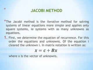
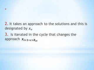
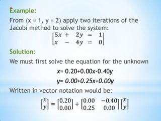
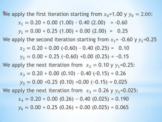
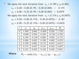
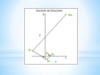
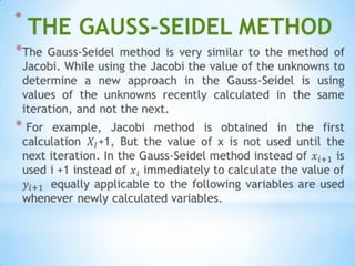
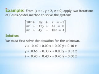
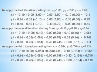
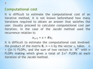
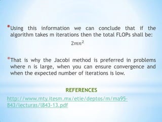
SlideShare a Scribd company logo
ITERATIVE METHODS FOR THE SOLUTION OF SYSTEM OF LINEAR EQUATIONS OSCAR EDUARDO MENDIVELSO OROZCO I studyPetroleumEngineering     Numerical Methods
JACOBI METHOD The Jacobi method is the iterative method for solving systems of linear equations more simple and applies only square systems, ie systems with as many unknowns as equations. First, we determine the equation of recurrence. For this order the equations and unknowns. Of the equation i cleared the unknown i. In matrix notation is written as: 𝒙=𝒄+𝑩𝒙      where x is the vector of unknowns.  
2.It takes an approach to the solutions and this is designated by 𝒙𝒐 3. Is iterated in the cycle that changes the approach  𝒙𝒊+𝟏=𝒄+𝑩𝒙𝒊  
Example: From (x = 1, y = 2) apply two iterations of the Jacobi method to solve the system:                                  𝟓𝒙 +𝟐𝒚  =𝟏𝒙    −𝟒𝒚  =𝟎 Solution: We must first solve the equation for the unknown x= 0.20+0.00x-0.40y 		y= 0.00+0.25x+0.00y Written in vector notation would be: 𝑥𝑦=0.200.00+0.00−0.400.250.00𝑥𝑦  
We apply the first iteration starting from𝑥0=1.00 y 𝑦0=2.00: 𝑥1=0.20 + 0.00 (1.00) - 0.40 (2.00)   = -0.60 𝑦1=0.00 + 0.25 (1.00) + 0.00 (2.00)  =   0.25 We apply the second iteration starting from 𝑥1= -0.60 y 𝑦1=0.25  𝑥2= 0.20 + 0.00 (-0.60) - 0.40 (0.25) =   0.10 𝑦2=0.00 + 0.25 (−0.60) +0.00 (0.25) = −0.15 We apply the next iteration from 𝑥2= 0.10 y 𝑦1=0.25: 𝑥3= 0.20 + 0.00 (0.10) - 0.40 (-0.15) = 0.26 𝑦3= 0.00 +0.25 (0.10) +0.00 (−0.15) = 0.025 We apply the next iteration from 𝑥3=0.26 y 𝑦3=0.025: 𝑥4=0.20 + 0.00 (0.26) − 0.40 (0.025) = 0.190 𝑦4=0.00 + 0.25 (0.26) + 0.00 (0.025) = 0.065  
     We apply the next iteration from 𝑥4=0.190 y 𝑦4=0.065: 𝑥5=0.20 + 0.00 (0.19) − 0.40 (0.065)   =    0.174 𝑦5=0.00 + 0.25 (0.19) + 0.00 (0.065)   =  0.0475     We apply the next iteration from  𝑥5=0.174 y 𝑦4=0.0475: 𝑥6=0.20 + 0.00 (0.174) − 0.40 (0.0475) =   0.181 𝑦6=0.00 + 0.25 (0.174) + 0.00 (0.0475) = 0.0435 Where  
THE GAUSS-SEIDEL METHOD The Gauss-Seidel method is very similar to the method of Jacobi. While using the Jacobi the value of the unknowns to determine a new approach in the Gauss-Seidel is using values of the unknowns recently calculated in the same iteration, and not the next. For example, Jacobi method is obtained in the first calculation 𝑋𝐼+1, But the value of x is not used until the next iteration. In the Gauss-Seidel method instead of 𝑥𝑖+1is used i +1 instead of 𝑥𝑖 immediatelyto calculate the value of 𝑦𝑖+1  equally applicable to the following variables are used whenever newly calculated variables.  
Example: From (x = 1, y = 2, z = 0) apply two iterations   of Gauss-Seidel method to solve the system: 10𝑥+0𝑦   +𝑧   =−14𝑥   +12𝑦 +4𝑧  =  84𝑥   +4𝑦    +10𝑧 = 4 Solution: We must first solve the equation for the unknown. x = −0.10 + 0.00 x + 0.00 y + 0.10 z 		y =  0.66  − 0.33 x + 0.00 y + 0.33 z z = 0.40 −0.40 x − 0.40 y + 0.00 z  
We apply the first iteration starting from𝑥0=1.00, 𝑦0=2.00 𝑦 𝑧=0.00: x1 = −0.10 + 0.00 (1.00) +  0.00 (2.00) +  0.10 (0.00) =  −0.1 	y1 = 0.66 − 0.33 (−0.10) +  0.00 (2.00) +  0.33 (0.00) =  0.70 z1 = 0.40 − 0.40(−0.10) − 0.40 (0.70) + 0.00 (0.00) = 0.16 We apply the second iteration starting from 𝑥1= -0.10, 𝑦1=0.70 y 𝑧1=0.16: x1 = −0.10 + 0.00(−0.10) + 0.00 (0.70) + 0.10 (0.16) = −0.084 y1 = 0.66 − 0.33(−0.084) + 0.00 (0.70) + 0.33 (0.16)  =  0.748 z1 = 0.40 − 0.40(−0.084) − 0.40 (0.748) + 0.00 (0.16) = 0.134 We apply the third iteration starting from 𝑥1= -0.084,  𝑦1=0.748 y 𝑧1=0.134: x1 = −0.10 +0.00(−0.084) +0.00(0.748) +0.10 (0.134) = −0.086 	y1 = 0.66 − 0.33(−0.086) + 0.00 (0.748) + 0.33 (0.134) = 0.740 z1 = 0.40 − 0.40(−0.086) − 0.40 (0.740) + 0.00 (0.134) = 0.138  
Computationalcost It is difficult to estimate the computational cost of an iterative method, it is not known beforehand how many iterations required to obtain an answer that satisfies the user. Usually proceed to calculate computational cost per iteration. In the case of the Jacobi method used the recurrence relation is: 𝒙𝒊+𝟏=𝐜+𝑩𝒙𝒊 It is difficult to estimate the computational cost involved: the product of the matrix B, n × n by the vector 𝑥𝑖 takes    n × (2n-1) FLOPs, and the sum of two vectors in ℜ𝑛  with n FLOPs making which gives a total of 2𝑛2 FLOPs at each iteration of the Jacobi method.   
Using this information we can conclude that if the algorithm takes m iterations then the total FLOPs shall be: 2𝑚𝑛2 That is why the Jacobi method is preferred in problems where n is large, when you can ensure convergence and when the expected number of iterations is low. REFERENCES http://www.mty.itesm.mx/etie/deptos/m/ma95-843/lecturas/l843-13.pdf  

More Related Content

What's hot

Linear algebra03fallleturenotes01
Linear algebra03fallleturenotes01Linear algebra03fallleturenotes01
Linear algebra03fallleturenotes01
ST ZULAIHA NURHAJARURAHMAH
 
Simple Linear Regression
Simple Linear RegressionSimple Linear Regression
Simple Linear Regression
Sindhu Rumesh Kumar
 
1605 power series
1605 power series1605 power series
1605 power series
Dr Fereidoun Dejahang
 
Lsd ee n
Lsd ee nLsd ee n
Lsd ee n
Asyraf Ghani
 
power series & radius of convergence
power series & radius of convergencepower series & radius of convergence
power series & radius of convergence
jigar sable
 
Series solutions airy's equation
Series solutions airy's equationSeries solutions airy's equation
Series solutions airy's equation
Tarun Gehlot
 
Power series & Radius of convergence
Power series & Radius of convergencePower series & Radius of convergence
Power series & Radius of convergence
Dhruv Darji
 
REGRESSION ANALYSIS
REGRESSION ANALYSISREGRESSION ANALYSIS
REGRESSION ANALYSIS
ONE Virtual Services
 
4.1 quadratic functions
4.1 quadratic functions4.1 quadratic functions
4.1 quadratic functions
morrobea
 
Power series and radius of convergence
Power series and radius of convergencePower series and radius of convergence
Power series and radius of convergence
Yashh Pandya
 
Calc 6.1b
Calc 6.1bCalc 6.1b
Calc 6.1b
hartcher
 
Series solution to ordinary differential equations
Series solution to ordinary differential equations Series solution to ordinary differential equations
Series solution to ordinary differential equations
University of Windsor
 
160280102042 c3 aem
160280102042 c3 aem160280102042 c3 aem
160280102042 c3 aem
L.D. COLLEGE OF ENGINEERING
 
170120107066 power series.ppt
170120107066 power series.ppt170120107066 power series.ppt
170120107066 power series.ppt
harsh kothari
 
Gauss jordan and Guass elimination method
Gauss jordan and Guass elimination methodGauss jordan and Guass elimination method
Gauss jordan and Guass elimination method
Meet Nayak
 
Physics o
Physics oPhysics o
Physics o
Jackie Buchanan
 
Ch6 series solutions algebra
Ch6 series solutions algebraCh6 series solutions algebra
Ch6 series solutions algebra
Asyraf Ghani
 
Solution of ordinary differential equetion
Solution of ordinary differential equetionSolution of ordinary differential equetion
Solution of ordinary differential equetion
Ardha Aslam
 
Solution of equations for methods iterativos
Solution of equations for methods iterativosSolution of equations for methods iterativos
Solution of equations for methods iterativos
DUBAN CASTRO
 

What's hot (19)

Linear algebra03fallleturenotes01
Linear algebra03fallleturenotes01Linear algebra03fallleturenotes01
Linear algebra03fallleturenotes01
 
Simple Linear Regression
Simple Linear RegressionSimple Linear Regression
Simple Linear Regression
 
1605 power series
1605 power series1605 power series
1605 power series
 
Lsd ee n
Lsd ee nLsd ee n
Lsd ee n
 
power series & radius of convergence
power series & radius of convergencepower series & radius of convergence
power series & radius of convergence
 
Series solutions airy's equation
Series solutions airy's equationSeries solutions airy's equation
Series solutions airy's equation
 
Power series & Radius of convergence
Power series & Radius of convergencePower series & Radius of convergence
Power series & Radius of convergence
 
REGRESSION ANALYSIS
REGRESSION ANALYSISREGRESSION ANALYSIS
REGRESSION ANALYSIS
 
4.1 quadratic functions
4.1 quadratic functions4.1 quadratic functions
4.1 quadratic functions
 
Power series and radius of convergence
Power series and radius of convergencePower series and radius of convergence
Power series and radius of convergence
 
Calc 6.1b
Calc 6.1bCalc 6.1b
Calc 6.1b
 
Series solution to ordinary differential equations
Series solution to ordinary differential equations Series solution to ordinary differential equations
Series solution to ordinary differential equations
 
160280102042 c3 aem
160280102042 c3 aem160280102042 c3 aem
160280102042 c3 aem
 
170120107066 power series.ppt
170120107066 power series.ppt170120107066 power series.ppt
170120107066 power series.ppt
 
Gauss jordan and Guass elimination method
Gauss jordan and Guass elimination methodGauss jordan and Guass elimination method
Gauss jordan and Guass elimination method
 
Physics o
Physics oPhysics o
Physics o
 
Ch6 series solutions algebra
Ch6 series solutions algebraCh6 series solutions algebra
Ch6 series solutions algebra
 
Solution of ordinary differential equetion
Solution of ordinary differential equetionSolution of ordinary differential equetion
Solution of ordinary differential equetion
 
Solution of equations for methods iterativos
Solution of equations for methods iterativosSolution of equations for methods iterativos
Solution of equations for methods iterativos
 

Viewers also liked

Jacobi and gauss-seidel
Jacobi and gauss-seidelJacobi and gauss-seidel
Jacobi and gauss-seidel
arunsmm
 
Directive-based approach to Heterogeneous Computing
Directive-based approach to Heterogeneous ComputingDirective-based approach to Heterogeneous Computing
Directive-based approach to Heterogeneous Computing
Ruymán Reyes
 
Jawaban uts astl ganjil analisa sistem tenaga
Jawaban uts astl ganjil analisa sistem tenagaJawaban uts astl ganjil analisa sistem tenaga
Jawaban uts astl ganjil analisa sistem tenaga
suparman unkhair
 
Iterative methods
Iterative methodsIterative methods
Iterative methods
Ketan Nayak
 
System of linear equations
System of linear equationsSystem of linear equations
System of linear equations
Diler4
 
Chapter 5
Chapter 5Chapter 5
Iterativos Methods
Iterativos MethodsIterativos Methods
Iterativos Methods
Jeannie
 
Iterative methods
Iterative methodsIterative methods
Iterative methods
rubenarismendi
 
Polycarbonates
PolycarbonatesPolycarbonates
Polycarbonates
hlksd
 
Linear equation in two variables
Linear equation in two variablesLinear equation in two variables
Linear equation in two variables
Abhaya Gupta
 
Es272 ch4a
Es272 ch4aEs272 ch4a
Nsm
Nsm Nsm
56 system of linear equations
56 system of linear equations56 system of linear equations
56 system of linear equations
alg1testreview
 
Iterative methods
Iterative methodsIterative methods
Iterative methods
Kt Silva
 
Linear Systems Gauss Seidel
Linear Systems   Gauss SeidelLinear Systems   Gauss Seidel
Linear Systems Gauss Seidel
Eric Davishahl
 
Gauss seidel
Gauss seidelGauss seidel
Gauss seidel
Ahmed M. Elkholy
 
NUMERICAL METHODS -Iterative methods(indirect method)
NUMERICAL METHODS -Iterative methods(indirect method)NUMERICAL METHODS -Iterative methods(indirect method)
NUMERICAL METHODS -Iterative methods(indirect method)
krishnapriya R
 
linear equation
linear equationlinear equation
linear equation
kanishkaanandkv
 
Java Exception handling
Java Exception handlingJava Exception handling
Java Exception handling
kamal kotecha
 
Finite difference method
Finite difference methodFinite difference method
Finite difference method
Divyansh Verma
 

Viewers also liked (20)

Jacobi and gauss-seidel
Jacobi and gauss-seidelJacobi and gauss-seidel
Jacobi and gauss-seidel
 
Directive-based approach to Heterogeneous Computing
Directive-based approach to Heterogeneous ComputingDirective-based approach to Heterogeneous Computing
Directive-based approach to Heterogeneous Computing
 
Jawaban uts astl ganjil analisa sistem tenaga
Jawaban uts astl ganjil analisa sistem tenagaJawaban uts astl ganjil analisa sistem tenaga
Jawaban uts astl ganjil analisa sistem tenaga
 
Iterative methods
Iterative methodsIterative methods
Iterative methods
 
System of linear equations
System of linear equationsSystem of linear equations
System of linear equations
 
Chapter 5
Chapter 5Chapter 5
Chapter 5
 
Iterativos Methods
Iterativos MethodsIterativos Methods
Iterativos Methods
 
Iterative methods
Iterative methodsIterative methods
Iterative methods
 
Polycarbonates
PolycarbonatesPolycarbonates
Polycarbonates
 
Linear equation in two variables
Linear equation in two variablesLinear equation in two variables
Linear equation in two variables
 
Es272 ch4a
Es272 ch4aEs272 ch4a
Es272 ch4a
 
Nsm
Nsm Nsm
Nsm
 
56 system of linear equations
56 system of linear equations56 system of linear equations
56 system of linear equations
 
Iterative methods
Iterative methodsIterative methods
Iterative methods
 
Linear Systems Gauss Seidel
Linear Systems   Gauss SeidelLinear Systems   Gauss Seidel
Linear Systems Gauss Seidel
 
Gauss seidel
Gauss seidelGauss seidel
Gauss seidel
 
NUMERICAL METHODS -Iterative methods(indirect method)
NUMERICAL METHODS -Iterative methods(indirect method)NUMERICAL METHODS -Iterative methods(indirect method)
NUMERICAL METHODS -Iterative methods(indirect method)
 
linear equation
linear equationlinear equation
linear equation
 
Java Exception handling
Java Exception handlingJava Exception handling
Java Exception handling
 
Finite difference method
Finite difference methodFinite difference method
Finite difference method
 

Similar to Iterative methods for the solution

numericai matmatic matlab uygulamalar ali abdullah
numericai matmatic  matlab  uygulamalar ali abdullahnumericai matmatic  matlab  uygulamalar ali abdullah
numericai matmatic matlab uygulamalar ali abdullah
Ali Abdullah
 
Mohammad shoaib babar
Mohammad shoaib babarMohammad shoaib babar
Mohammad shoaib babar
MOHAMMADBABAR13
 
system of algebraic equation by Iteration method
system of algebraic equation by Iteration methodsystem of algebraic equation by Iteration method
system of algebraic equation by Iteration method
Akhtar Kamal
 
engineeringmathematics-iv_unit-v
engineeringmathematics-iv_unit-vengineeringmathematics-iv_unit-v
engineeringmathematics-iv_unit-v
Kundan Kumar
 
Engineering Mathematics-IV_B.Tech_Semester-IV_Unit-V
Engineering Mathematics-IV_B.Tech_Semester-IV_Unit-VEngineering Mathematics-IV_B.Tech_Semester-IV_Unit-V
Engineering Mathematics-IV_B.Tech_Semester-IV_Unit-V
Rai University
 
Schwarzchild solution derivation
Schwarzchild solution derivationSchwarzchild solution derivation
Schwarzchild solution derivation
Hassaan Saleem
 
Neural network - how does it work - I mean... literally!
Neural network - how does it work - I mean... literally!Neural network - how does it work - I mean... literally!
Neural network - how does it work - I mean... literally!
Christoph Diefenthal
 
Study Material Numerical Solution of Odinary Differential Equations
Study Material Numerical Solution of Odinary Differential EquationsStudy Material Numerical Solution of Odinary Differential Equations
Study Material Numerical Solution of Odinary Differential Equations
Meenakshisundaram N
 
U3 10 sistemas de ecuaciones
U3   10 sistemas de ecuacionesU3   10 sistemas de ecuaciones
U3 10 sistemas de ecuaciones
UNEFA Zulia
 
Class 10 maths
Class 10 maths Class 10 maths
Class 10 maths
Bhaskar goyal
 
Ecuaciones lineales de orden superior
Ecuaciones lineales de orden superiorEcuaciones lineales de orden superior
Ecuaciones lineales de orden superior
mariarivas114
 
PO_groupVI_Term assignment.pptx
PO_groupVI_Term assignment.pptxPO_groupVI_Term assignment.pptx
PO_groupVI_Term assignment.pptx
PATELPUNIT2
 
Calculas
CalculasCalculas
Calculas
Vatsal Manavar
 
Sistempertidaksamaanduavariabel2122
Sistempertidaksamaanduavariabel2122Sistempertidaksamaanduavariabel2122
Sistempertidaksamaanduavariabel2122
Franxisca Kurniawati
 
System of equations
System of equationsSystem of equations
System of equations
mariacadena
 
System of equations
System of equationsSystem of equations
System of equations
mariacadena
 
System of equations
System of equationsSystem of equations
System of equations
mariacadena
 
System of equations
System of equationsSystem of equations
System of equations
mariacadena
 
System of equations
System of equationsSystem of equations
System of equations
mariacadena
 
Lecture 3
Lecture 3Lecture 3
Lecture 3
RajKumar382958
 

Similar to Iterative methods for the solution (20)

numericai matmatic matlab uygulamalar ali abdullah
numericai matmatic  matlab  uygulamalar ali abdullahnumericai matmatic  matlab  uygulamalar ali abdullah
numericai matmatic matlab uygulamalar ali abdullah
 
Mohammad shoaib babar
Mohammad shoaib babarMohammad shoaib babar
Mohammad shoaib babar
 
system of algebraic equation by Iteration method
system of algebraic equation by Iteration methodsystem of algebraic equation by Iteration method
system of algebraic equation by Iteration method
 
engineeringmathematics-iv_unit-v
engineeringmathematics-iv_unit-vengineeringmathematics-iv_unit-v
engineeringmathematics-iv_unit-v
 
Engineering Mathematics-IV_B.Tech_Semester-IV_Unit-V
Engineering Mathematics-IV_B.Tech_Semester-IV_Unit-VEngineering Mathematics-IV_B.Tech_Semester-IV_Unit-V
Engineering Mathematics-IV_B.Tech_Semester-IV_Unit-V
 
Schwarzchild solution derivation
Schwarzchild solution derivationSchwarzchild solution derivation
Schwarzchild solution derivation
 
Neural network - how does it work - I mean... literally!
Neural network - how does it work - I mean... literally!Neural network - how does it work - I mean... literally!
Neural network - how does it work - I mean... literally!
 
Study Material Numerical Solution of Odinary Differential Equations
Study Material Numerical Solution of Odinary Differential EquationsStudy Material Numerical Solution of Odinary Differential Equations
Study Material Numerical Solution of Odinary Differential Equations
 
U3 10 sistemas de ecuaciones
U3   10 sistemas de ecuacionesU3   10 sistemas de ecuaciones
U3 10 sistemas de ecuaciones
 
Class 10 maths
Class 10 maths Class 10 maths
Class 10 maths
 
Ecuaciones lineales de orden superior
Ecuaciones lineales de orden superiorEcuaciones lineales de orden superior
Ecuaciones lineales de orden superior
 
PO_groupVI_Term assignment.pptx
PO_groupVI_Term assignment.pptxPO_groupVI_Term assignment.pptx
PO_groupVI_Term assignment.pptx
 
Calculas
CalculasCalculas
Calculas
 
Sistempertidaksamaanduavariabel2122
Sistempertidaksamaanduavariabel2122Sistempertidaksamaanduavariabel2122
Sistempertidaksamaanduavariabel2122
 
System of equations
System of equationsSystem of equations
System of equations
 
System of equations
System of equationsSystem of equations
System of equations
 
System of equations
System of equationsSystem of equations
System of equations
 
System of equations
System of equationsSystem of equations
System of equations
 
System of equations
System of equationsSystem of equations
System of equations
 
Lecture 3
Lecture 3Lecture 3
Lecture 3
 

Iterative methods for the solution

  • 1. ITERATIVE METHODS FOR THE SOLUTION OF SYSTEM OF LINEAR EQUATIONS OSCAR EDUARDO MENDIVELSO OROZCO I studyPetroleumEngineering Numerical Methods
  • 2. JACOBI METHOD The Jacobi method is the iterative method for solving systems of linear equations more simple and applies only square systems, ie systems with as many unknowns as equations. First, we determine the equation of recurrence. For this order the equations and unknowns. Of the equation i cleared the unknown i. In matrix notation is written as: 𝒙=𝒄+𝑩𝒙 where x is the vector of unknowns.  
  • 3. 2.It takes an approach to the solutions and this is designated by 𝒙𝒐 3. Is iterated in the cycle that changes the approach  𝒙𝒊+𝟏=𝒄+𝑩𝒙𝒊  
  • 4. Example: From (x = 1, y = 2) apply two iterations of the Jacobi method to solve the system:                                𝟓𝒙 +𝟐𝒚  =𝟏𝒙    −𝟒𝒚  =𝟎 Solution: We must first solve the equation for the unknown x= 0.20+0.00x-0.40y y= 0.00+0.25x+0.00y Written in vector notation would be: 𝑥𝑦=0.200.00+0.00−0.400.250.00𝑥𝑦  
  • 5. We apply the first iteration starting from𝑥0=1.00 y 𝑦0=2.00: 𝑥1=0.20 + 0.00 (1.00) - 0.40 (2.00) = -0.60 𝑦1=0.00 + 0.25 (1.00) + 0.00 (2.00) = 0.25 We apply the second iteration starting from 𝑥1= -0.60 y 𝑦1=0.25 𝑥2= 0.20 + 0.00 (-0.60) - 0.40 (0.25) = 0.10 𝑦2=0.00 + 0.25 (−0.60) +0.00 (0.25) = −0.15 We apply the next iteration from 𝑥2= 0.10 y 𝑦1=0.25: 𝑥3= 0.20 + 0.00 (0.10) - 0.40 (-0.15) = 0.26 𝑦3= 0.00 +0.25 (0.10) +0.00 (−0.15) = 0.025 We apply the next iteration from 𝑥3=0.26 y 𝑦3=0.025: 𝑥4=0.20 + 0.00 (0.26) − 0.40 (0.025) = 0.190 𝑦4=0.00 + 0.25 (0.26) + 0.00 (0.025) = 0.065  
  • 6. We apply the next iteration from 𝑥4=0.190 y 𝑦4=0.065: 𝑥5=0.20 + 0.00 (0.19) − 0.40 (0.065) = 0.174 𝑦5=0.00 + 0.25 (0.19) + 0.00 (0.065) = 0.0475 We apply the next iteration from 𝑥5=0.174 y 𝑦4=0.0475: 𝑥6=0.20 + 0.00 (0.174) − 0.40 (0.0475) = 0.181 𝑦6=0.00 + 0.25 (0.174) + 0.00 (0.0475) = 0.0435 Where  
  • 7.
  • 8. THE GAUSS-SEIDEL METHOD The Gauss-Seidel method is very similar to the method of Jacobi. While using the Jacobi the value of the unknowns to determine a new approach in the Gauss-Seidel is using values of the unknowns recently calculated in the same iteration, and not the next. For example, Jacobi method is obtained in the first calculation 𝑋𝐼+1, But the value of x is not used until the next iteration. In the Gauss-Seidel method instead of 𝑥𝑖+1is used i +1 instead of 𝑥𝑖 immediatelyto calculate the value of 𝑦𝑖+1  equally applicable to the following variables are used whenever newly calculated variables.  
  • 9. Example: From (x = 1, y = 2, z = 0) apply two iterations of Gauss-Seidel method to solve the system: 10𝑥+0𝑦   +𝑧   =−14𝑥   +12𝑦 +4𝑧  =  84𝑥   +4𝑦    +10𝑧 = 4 Solution: We must first solve the equation for the unknown. x = −0.10 + 0.00 x + 0.00 y + 0.10 z y = 0.66 − 0.33 x + 0.00 y + 0.33 z z = 0.40 −0.40 x − 0.40 y + 0.00 z  
  • 10. We apply the first iteration starting from𝑥0=1.00, 𝑦0=2.00 𝑦 𝑧=0.00: x1 = −0.10 + 0.00 (1.00) + 0.00 (2.00) + 0.10 (0.00) = −0.1 y1 = 0.66 − 0.33 (−0.10) + 0.00 (2.00) + 0.33 (0.00) = 0.70 z1 = 0.40 − 0.40(−0.10) − 0.40 (0.70) + 0.00 (0.00) = 0.16 We apply the second iteration starting from 𝑥1= -0.10, 𝑦1=0.70 y 𝑧1=0.16: x1 = −0.10 + 0.00(−0.10) + 0.00 (0.70) + 0.10 (0.16) = −0.084 y1 = 0.66 − 0.33(−0.084) + 0.00 (0.70) + 0.33 (0.16) = 0.748 z1 = 0.40 − 0.40(−0.084) − 0.40 (0.748) + 0.00 (0.16) = 0.134 We apply the third iteration starting from 𝑥1= -0.084,  𝑦1=0.748 y 𝑧1=0.134: x1 = −0.10 +0.00(−0.084) +0.00(0.748) +0.10 (0.134) = −0.086 y1 = 0.66 − 0.33(−0.086) + 0.00 (0.748) + 0.33 (0.134) = 0.740 z1 = 0.40 − 0.40(−0.086) − 0.40 (0.740) + 0.00 (0.134) = 0.138  
  • 11. Computationalcost It is difficult to estimate the computational cost of an iterative method, it is not known beforehand how many iterations required to obtain an answer that satisfies the user. Usually proceed to calculate computational cost per iteration. In the case of the Jacobi method used the recurrence relation is: 𝒙𝒊+𝟏=𝐜+𝑩𝒙𝒊 It is difficult to estimate the computational cost involved: the product of the matrix B, n × n by the vector 𝑥𝑖 takes n × (2n-1) FLOPs, and the sum of two vectors in ℜ𝑛  with n FLOPs making which gives a total of 2𝑛2 FLOPs at each iteration of the Jacobi method.  
  • 12. Using this information we can conclude that if the algorithm takes m iterations then the total FLOPs shall be: 2𝑚𝑛2 That is why the Jacobi method is preferred in problems where n is large, when you can ensure convergence and when the expected number of iterations is low. REFERENCES http://www.mty.itesm.mx/etie/deptos/m/ma95-843/lecturas/l843-13.pdf