The bisection method is a numerical technique for finding roots of equations by repeatedly bisecting an interval where a function changes sign. This method requires a closed interval [a,b] such that f(a) and f(b) have opposite signs, and it continues halving the interval until the length is less than a predefined error threshold. The algorithm is straightforward, allowing for precise estimation of the root through calculated iterations until the desired accuracy is achieved.
![Bisection Method
The bisection method (sometimes called the midpoint method for equations) is a
method used to estimate the solution of an equation.
Like the Regula-Falsi Method (and others) we approach this problem by writing
the equation in the form f(x) = 0 for some function f(x). This reduces the problem
to finding a root for the function f(x).
Like the Regula-Falsi Method the Bisection Method also needs a closed interval
[a,b] for which the function f(x) is positive at one endpoint and negative at the
other. In other words f(x) must satisfy the condition f(a)⋅f(b) < 0. This means that
this algorithm can not be applied to find tangential roots.
There are several advantages that the Bisection method has over the Regula-
Falsi Method.
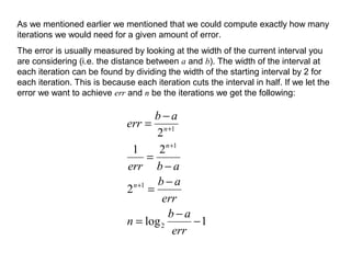
The number of steps required to estimate the root within the desired error
can be easily computed before the algorithm is applied. This gives a way to
compute how long the algorithm will compute. (Real-time applications)
The way that you get the next point is a much easier computation than how
you get the regula-falsi point (rfp).](https://image.slidesharecdn.com/bisectdn2-2-171003200120/85/Bisection-method-in-maths-4-2-320.jpg)
![Definition:-
• Given a closed interval [a,b] on which f changes sign, we
divide the interval in half and note that f must change
sign on either the right or the left half (or be zero at the
midpoint of [a,b].) We then replace [a,b] by the half-
interval on which f changes sign. This process is
repeated until the interval has total length less than
E(error) . In the end we have a closed interval of length
less than E on which f changes sign. The IVT
guarantees that there is a zero of f in this interval. The
endpoints of this interval, which are known, must be
within of this zero.](https://image.slidesharecdn.com/bisectdn2-2-171003200120/85/Bisection-method-in-maths-4-3-320.jpg)
![Bisection Algorithm
The idea for the Bisection Algorithm is to cut the interval [a,b] you are given in half
(bisect it) on each iteration by computing the midpoint xmid. The midpoint will
replace either a or b depending on if the sign of f(xmid) agrees with f(a) or f(b).
Step 1: Compute xmid = (a+b)/2
Step 2: If sign(f(xmid)) = 0 then end algorithm
else If sign(f(xmid)) = sign(f(a)) then a = xmid
else b = xmid
Step 3: Return to step 1
f(a)
f(b)
a b
root
xmid This shows how the points a, b
and xmid are related.
f(x)](https://image.slidesharecdn.com/bisectdn2-2-171003200120/85/Bisection-method-in-maths-4-4-320.jpg)
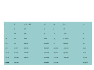
![Lets apply the Bisection Method to the same function as we did for the Regula-
Falsi Method. The equation is: x3
-2x-3=0, the function is: f(x)=x3
-2x-3.
This function has a root on the interval [0,2]
Iteration
a b xmid f(a) f(b) f(xmid)
1 0 2 1 -3 1 -4
2 1 2 1.5 -4 1 -2.262
3 1.5 2 1.75 -2.262 1 -1.140
4 1.75 2 1.875 -1.140 1 -.158](https://image.slidesharecdn.com/bisectdn2-2-171003200120/85/Bisection-method-in-maths-4-5-320.jpg)
![Example 1
Starting with the interval [1,2], find srqt(2) to within
two decimal places (to within an error of .01). The
function involved is f(x) = x2
-2. The following table
steps through the iteration until the size of the
interval, given in the last column, is less than .01.
The final result is the approximation 1.41406 for
the sqrt(2). This is guaranteed by the algorithm to
be within .01 (actually, to within 1/128) of sqrt(2).
In reality it agrees with sqrt(2) to three decimal
places, not just two.](https://image.slidesharecdn.com/bisectdn2-2-171003200120/85/Bisection-method-in-maths-4-7-320.jpg)
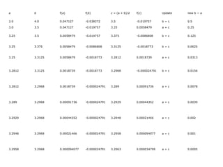
![Example 2
•Consider finding the root of f(x) = e-x
(3.2 sin(x)
- 0.5 cos(x)) on the interval [3, 4], this time
with εstep = 0.001, εabs = 0.001.
•Table 1. Bisection method applied to f(x) = e-
x
(3.2 sin(x) - 0.5 cos(x)).](https://image.slidesharecdn.com/bisectdn2-2-171003200120/85/Bisection-method-in-maths-4-9-320.jpg)


![CH-2_5 ROOTS_OF_NON_LINEAR_EQ [Compatibility Mode].pdf](https://cdn.slidesharecdn.com/ss_thumbnails/ch-25rootsofnonlineareqcompatibilitymode-260123171244-4215d39d-thumbnail.jpg?width=640&height=640&fit=bounds)


