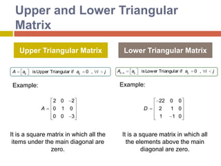
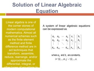
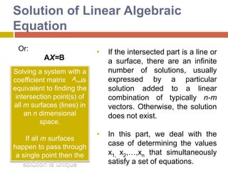
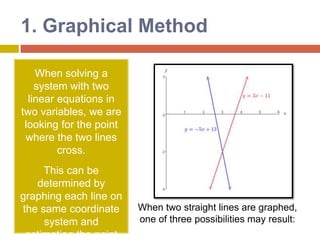
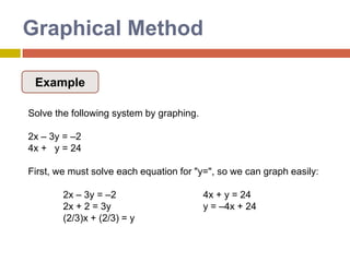
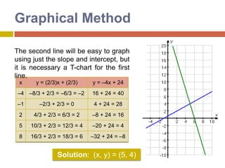
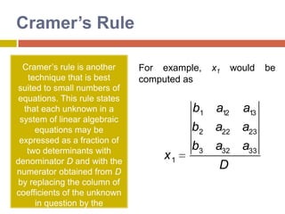
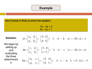
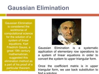
This document discusses various direct methods for solving linear systems of equations, including graphical methods, Cramer's rule, elimination of unknowns, Gaussian elimination, Gaussian-Jordan elimination, and LU decomposition. It provides examples and explanations of each method. Graphical methods can solve systems of 2 equations visually by plotting the lines. Cramer's rule uses determinants to find solutions. Elimination of unknowns combines equations to remove variables. Gaussian elimination converts the matrix to upper triangular form. Gaussian-Jordan elimination converts it to an identity matrix. LU decomposition factors the matrix into lower and upper triangular matrices.

1. DirectMethodstothesolution of linear equationssystemsLizeth Paola Barrero RiañoNumericalMethods – Industrial Univesity of Santander

2. SymmetricMatrix

3. TransposesMatrix

4. Determinant

5. Upper Triangular Matrix

6. Lower Triangular Matrix

7. BandedMatrix

8. AugmentedMatrix

9. MatrixMultiplicationBASIC FUNDAMENTALS

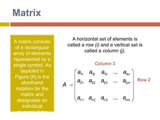
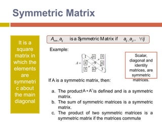
10. MatrixA horizontal set of elements is called a row(i) and a vertical set is called a column (j). A matrix consists of a rectangular array of elements represented by a single symbol. As depicted in Figure [A] is the shorthand notation for the matrix and designates an individual element of the matrix.Column 3Row 2

11. SymmetricMatrixIt is a square matrix in which the elements are symmetric about the main diagonalExample:Scalar, diagonal and identity matrices, are symmetric matrices.If A is a symmetric matrix, then:The product is defined and is a symmetric matrix.The sum of symmetric matrices is a symmetric matrix.The product of two symmetric matrices is a symmetric matrix if the matrices commute

12. TransposesMatrixLetanymatrix A=(aij) of mxnorder, thematrix B=(bij) de ordernxmisthe A transposeifthe A rows are the B columns . This operation is usually denoted by At = A' = BExample:Properties:

13. DeterminantGiven a square matrix A of n size, its determinant is defined as the sum of the any matrix line elements product (row or column) chosen, by their corresponding attachments.Example:

14. Determinant PropertiesIf a matrix has a line (row or column) of zeros, the determinant is zero.If a matrix has two equal rows or proportional, the determinant is nullIf we permute two parallels lines of a square matrix, its determinant changes sign.If we multiply all elements of a determinant line by a number, the determinant is multiplied by that number.If a matrix line is added another line multiplied by a number, the determinant does not change.The determinant of a matrix is equal to its transpose,If A has inverse matrix, A-1, it is verified that:

15. Upper and Lower Triangular MatrixUpper Triangular MatrixLower Triangular MatrixExample:Example:It is a square matrix in which all the items under the main diagonal are zero.It is a square matrix in which all the elements above the main diagonal are zero.

16. BandedMatrixA band matrix is a sparse matrix whose non-zero entries are confined to a diagonal band, comprising the main diagonal and zero or more diagonals on either side.Example:DiagonalTriadiagonalPentadiagonal

17. AugmentedMatrixIt is called extended or augmented matrix that is formed by the coefficient matrix and the vector of independent terms, which are usually separated with a dotted lineExample:

18. MatrixMultiplication.To define A ⋅ B is necessary that the number of columns in the first matrix coincides with the number of rows in the second matrix. The product order is given by the number of rows in the first matrix per the number of columns in the second matrix. That is, if A is mxn order and B is nxp order, then C = A ⋅ B is mxp order.theproduct A.BisGivenanothermatrixin whicheachCijisthenthrowproduct of A per thenthcolumn of B, namelytheelement

19. Matrix MultiplicationGraphically:Example:

20. Solution of Linear Algebraic EquationLinear algebra is one of the corner stones of modern computational mathematics. Almost all numerical schemes such as the finite element method and finite difference method are in act techniques that transform, assemble, reduce, rearrange, and/or approximate the differential, integral, or other types of equations to systems of linear algebraic equations.A system of linear algebraic equations can be expressed as

21. Solution of Linear Algebraic EquationOr:AX=BIf the intersected part is a line or a surface, there are an infinite number of solutions, usually expressed by a particular solution added to a linear combination of typically n-m vectors. Otherwise, the solution does not exist.

22. In this part, we deal with the case of determining the values x1, x2,…,xn that simultaneously satisfy a set of equations.Solving a system with a coefficient matrix is equivalent to finding the intersection point(s) of all m surfaces (lines) in an n dimensional space. If all m surfaces happen to pass through a single point then the solution is unique

23. Small Systems of Linear EquationsGraphicalMethodCramer’s RuleTheElimination of Unknows

24. 1. Graphical MethodWhen solving a system with two linear equations in two variables, we are looking for the point where the two lines cross. This can be determined by graphing each line on the same coordinate system and estimating the point of intersection.When two straight lines are graphed, one of three possibilities may result:

25. Graphical MethodWhen two lines cross in exactly one point, the system is consistent and independent and the solution is the one ordered pair where the two lines cross. The coordinates of this ordered pair can be estimated from the graph of the two lines:Case 1Independent system:one solution point

26. Graphical MethodThis graph shows two distinct lines that are parallel. Since parallel lines never cross, then there can be no intersection; that is, for a system of equations that graphs as parallel lines, there can be no solution. This is called an "inconsistent" system of equations, and it has no solution.Case 2Inconsistent system:no solution andno intersection point

27. Graphical MethodThis graph appears to show only one line. Actually, it is the same line drawn twice. These "two" lines, really being the same line, "intersect" at every point along their length. This is called a "dependent" system, and the "solution" is the whole line.Case 3Dependent system:the solution is thewhole line

28. Graphical MethodADVANTAGES:The graphical method is good because it clearly illustrates the principle involved. DISADVANTAGES:It does not always give us an exact solution.

29. It cannot be used when we have more than two variables in the equations. For instance, if the lines cross at a shallow angle it can be just about impossible to tell where the lines cross:

30. Graphical MethodExampleSolve the following system by graphing. 2x – 3y = –24x + y = 24First, we must solve each equation for "y=", so we can graph easily: 2x – 3y = –2 4x + y = 24 2x + 2 = 3y y = –4x + 24 (2/3)x + (2/3) = y

31. Graphical MethodThe second line will be easy to graph using just the slope and intercept, but it is necessary a T-chart for the first line.Solution: (x, y) = (5, 4)

32. Cramer’s RuleCramer’s rule is another technique that is best suited to small numbers of equations. This rule states that each unknown in a system of linear algebraic equations may be expressed as a fraction of two determinants with denominator D and with the numerator obtained from D by replacing the column of coefficients of the unknown in question by the constants b1, b2, … ,bn. For example, x1would be computed as

33. ExampleUse Cramer’s Rule to solve the system: 5x – 4y = 26x – 5y = 1Solution:Webeginbysetting up and evaluatingthethreedeterminants:

34. ExampleFromCramer’s Rule, wehave:andThesolutionis (6,7)Cramer’s Rule doesnotapplyif D=0. When D=0 , thesystemiseitherinconsistentordependent. Anothermethodmustbeusedtosolveit.

35. TheElimination of UnknowsThe elimination of unknowns by combing equations is an algebraic approach that can be illustrated for a set of two equations:The basic strategy is to multiply the equations by constants so that of the unknowns will be eliminated when the two equations are combined. The result is a single equation that can be solved for the remaining unknown. This value can then be substituted into either of the original equations to compute the other variable.For example, these equations might be multiplied by a21 and a11 to give

36. TheElimination of UnknowsSubtracting Eq. 3 from 4 will, therefore, eliminate the xt term from the equations to yieldWhich can be solve forThis equation can then be substituted into Eq. 1, which can be solved for

37. TheElimination of UnknowsNotice that these equations follow directly from Cramer’s rule, which statesEXAMPLEUse the elimination of unknown to solve,

38. GaussianEliminationGaussian Elimination is considered the workhorse of computational science for the solution of a system of linear equations. Karl Friedrich Gauss, a great 19th century mathematician, suggested this elimination method as a part of his proof of a particular theorem. Computational scientists use this “proof” as a direct computational method. Gaussian Elimination is a systematic application of elementary row operations to a system of linear equations in order to convert the system to upper triangular form. Once the coefficient matrix is in upper triangular form, we use back substitution to find a solution.

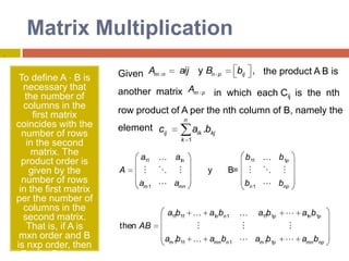
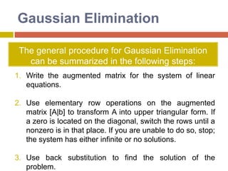
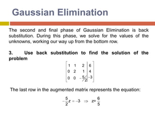
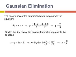
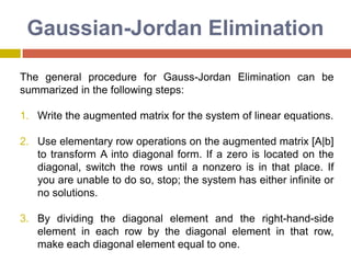
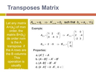
39. GaussianEliminationThe general procedure for Gaussian Elimination can be summarized in the following steps: Write the augmented matrix for the system of linear equations. Use elementary row operations on the augmented matrix [A|b] to transform A into upper triangular form. If a zero is located on the diagonal, switch the rows until a nonzero is in that place. If you are unable to do so, stop; the system has either infinite or no solutions. Use back substitution to find the solution of the problem.

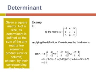
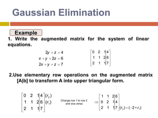
40. GaussianEliminationExample1. Write the augmented matrix for the system of linear equations.2.Use elementary row operations on theaugmented matrix [A|b] to transform A into upper triangular form.Change row 1 to row 2and vice versa

41. GaussianEliminationNotice that the original coefficient matrix had a “0” on the diagonal in row 1. Since we needed to use multiples of that diagonal element to eliminate the elements below it, we switched two rows in order to move a nonzero element into that position. We can use the same technique when a “0” appears on the diagonal as a result of calculation. If it is not possible to move a nonzero onto the diagonal by interchanging rows, then the system has either infinitely many solutions or no solution, and the coefficient matrix is said to be singular. Since all of the nonzero elements are now located in the “upper triangle” of the matrix, we have completed the first phase of solving a system of linear equations using Gaussian Elimination.

42. GaussianEliminationThe second and final phase of Gaussian Elimination is back substitution. During this phase, we solve for the values of the unknowns, working our way up from the bottom row. 3. Use back substitution to find the solution of the problemThe last row in the augmented matrix represents the equation:

43. GaussianEliminationThe second row of the augmented matrix represents the equation:Finally, the first row of the augmented matrix represents the equation

44. Gaussian-Jordan EliminationAs in Gaussian Elimination, again we are transforming the coefficient matrix into another matrix that is much easier to solve, and the system represented by the new augmented matrix has the same solution set as the original system of linear equations. In Gauss-Jordan Elimination, the goal is to transform the coefficient matrix into a diagonal matrix, and the zeros are introduced into the matrix one column at a time. We work to eliminate the elements both above and below the diagonal element of a given column in one pass through the matrix.

45. Gaussian-Jordan EliminationThe general procedure for Gauss-Jordan Elimination can be summarized in the following steps: Write the augmented matrix for the system of linear equations. Use elementary row operations on the augmented matrix [A|b] to transform A into diagonal form. If a zero is located on the diagonal, switch the rows until a nonzero is in that place. If you are unable to do so, stop; the system has either infinite or no solutions. By dividing the diagonal element and the right-hand-side element in each row by the diagonal element in that row, make each diagonal element equal to one.

46. Gaussian-Jordan EliminationExampleWe will apply Gauss-Jordan Elimination to the same example that was used to demonstrate Gaussian Elimination1-Write the augmented matrix for the system of linear equations.2. Use elementary row operations on the augmented matrix [A|b] to transform A into diagonal form.

47. Gaussian-Jordan Elimination3-By dividing the diagonal element and the right-hand-side element in each row by the diagonal element in that row, make each diagonal element equal to one.Notice that the coefficient matrix is now a diagonal matrix with ones on the diagonal. This is a special matrix called the identity matrix.

48. LU DecompositionJust as was the case with Gauss elimination, Lu decomposition requires pivoting to avoid division by zero. However, to simplify the following description, we will defer the issue of pivoting until after the fundamental approach is elaborated. In addition, the following explanation is limited to a set of three simultaneous equations. The results can be directly extended to n-dimensional systems.method.

49. Bibliographyhttp://www.purplemath.comhttp://ceee.rice.edu/Books