3 capitulo-iii-matriz-asociada-sem-13-t-l-c

CAPÍTULO III
MATRIZ ASOCIADA A UNA TRANSFORMACIÓN LINEAL.
CONTENIDO:
3.1 Matriz asociada a una transformación lineal.
3.2 Algebra de transformaciones lineales.
3.3 Composición de Transformaciones lineales.
3.4 Transformaciones lineales invertibles.
3.5 Teorema de equivalencias de una transformación lineal.
3.6 Isomorfismo inducido por una transformación lineal.
3.7 Cambio de base y semejanza de matrices.
3.8 Producto Interno. Definición. Teoremas de caracterización.
3.9 Norma de un Vector.
3.10 Ortogonalidad. Conjunto ortogonal y conjunto ortonormal.
3.11 Proceso de ortogonalidad de Gram Schmitdt.
3.12 Espacio Dual de un espacio vectorial.
3.13 Adjunta de una transformación lineal

88
3.3 COMPOSICIÓN DE TRANSFORMACIONES LINEALES. O PRODUCTO DE
TRANSFORMACIONES LINEALES.
DEFINICIÓN.Sean(𝑉;𝐾,+; ∙),(𝑊;𝐾,+; ∙) y (𝑈; 𝐾, +; ∙) espacios vectoriales y sean 𝑇1: 𝑉 → 𝑊y
𝑇2:𝑊 → 𝑈 dos transformaciones lineales. La aplicación composición 𝑇2o𝑇1:𝑉 → 𝑈 se define
como (𝑇2o𝑇1)(𝑋) = 𝑇2[𝑇1(𝑋)], ∀ 𝑋 ∈ 𝑉.
NOTA 1:La expresión 𝑇2o𝑇1 se lee: “Composición de 𝑇1 con 𝑇2” o también “𝑇2 compuesta con
𝑇1”
NOTA 2: La composición se puede generalizar para todas las transformaciones lineales entre
los espacios vectoriales: 𝑇𝑖 ∈ 𝐿(𝑉;𝑊) y 𝑇𝑗 ∈ 𝐿(𝑊;𝑈)
OBSERVACIÓN.La composición 𝑇2o𝑇1 es posible cuando la dimensión del espacio de llegada de
𝑇1 es igual a la dimensión del espacio de partida de 𝑇2 .
La composición 𝑇1o𝑇2 es posible cuando la dimensión del espacio de llegada de 𝑇2 es igual a la
dimensión del espacio de partida de 𝑇1 .
(𝑉; 𝐾, +; ∙) (𝑊;𝐾,+; ∙) (𝑈;𝐾,+; ∙)
𝑋 . 𝑇1(𝑋) . . 𝑇2[𝑇1(𝑋)] = (𝑇2o 𝑇1 )(𝑋)
𝑇2o 𝑇1
𝑇2
𝑇1
>
>
(𝑉; 𝐾, +; ∙) (𝑊;𝐾,+; ∙) (𝑈;𝐾,+; ∙)
𝑋 . 𝑇𝑖(𝑋) . . 𝑇𝑗[𝑇𝑖(𝑋)] = 𝑇𝑗o 𝑇𝑖 (𝑋)
𝑇𝑗o 𝑇𝑖
𝑇𝑗
𝑇𝑖
>
>
(𝑉𝑛
; 𝐾+; ∙) (𝑊𝑚
; 𝐾+; ∙) (𝑈𝑝
;𝐾+; ∙)
𝑇2𝑜𝑇1
𝑇1 𝑇2
(𝑉𝑛
; 𝐾+; ∙) (𝑊𝑚
; 𝐾+; ∙) (𝑈𝑝
;𝐾+; ∙)
𝑇𝑗𝑜𝑇𝑖
𝑇𝑖 𝑇𝑗

89
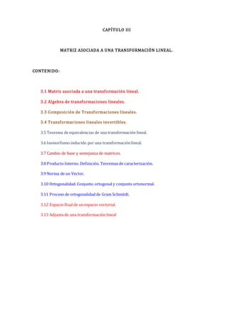
TEOREMA. La aplicación composición de dos transformaciones lineales 𝑇2o 𝑇1 es una
transformación lineal.
Demostración.
Sean las transformaciones lineales dadas en la definición y sea 𝑘1; 𝑘2 ∈ 𝐾 y 𝑋1; 𝑋2 ∈ 𝑉.
(𝑇2o 𝑇1)(𝑘1𝑋1 + 𝑘2𝑋2) = 𝑘1(𝑇2o 𝑇1)(𝑋1 ) + 𝑘2(𝑇2o 𝑇1)(𝑋2) ¡Probar!
En efecto:
(𝑇2o 𝑇1)(𝑘1𝑋1 + 𝑘2𝑋2)
= 𝑇2[𝑇1(𝑘1𝑋1 + 𝑘2𝑋2)] Por definición de composición
= 𝑇2[𝑇1(𝑘1𝑋1) + 𝑇1(𝑘2𝑋2)] Pues 𝑇1 es una T. L.
= 𝑇2[𝑘1𝑇1(𝑋1) + 𝑘2𝑇1(𝑋2)] Pues 𝑇1 es una T. L.
= 𝑇2[𝑘1𝑇1(𝑋1)] + 𝑇2[𝑘2𝑇1(𝑋2)] Pues 𝑇2 es una T. L.
= 𝑘1𝑇2[𝑇1(𝑋1)] + 𝑘2𝑇2[𝑇1(𝑋2)] Pues 𝑇2 es una T. L.
= 𝑘1(𝑇2o 𝑇1)(𝑋1) + 𝑘2(𝑇2o 𝑇1)(𝑋2) Por definición de Composición
Por lo tanto, la composición 𝑇2o 𝑇1 es una transformación lineal.
PROPOSICIÓN.Lamatrizasociadaalacomposicióndelastransformacioneslineales𝑇2o𝑇1:𝑉 →
𝑈, siendo 𝑇1:𝑉 → 𝑊 con matriz asociada 𝐴𝑇
1
y 𝑇2:𝑊 → 𝑈 con matriz asociada es dada 𝐴𝑇2
; es
dada por la matriz producto 𝐴𝑇2𝑜𝑇1
= [𝐴𝑇
2
][𝐴𝑇1
]
Prueba. Ejercicio.
PROPOSICIÓN. Para toda 𝑇𝑖 ∈ 𝐿(𝑉; 𝑊) y para todas las 𝑇𝑗 ;𝑇𝑚 ∈ 𝐿(𝑊;𝑍) se cumple que:
𝑇𝑗 + 𝑇𝑚 𝑜𝑇𝑖 = 𝑇𝑗𝑜𝑇𝑖 + 𝑇𝑚𝑜𝑇𝑖
(𝑉𝑛
; 𝐾+; ∙) (𝑊𝑚
; 𝐾+; ∙) (𝑈𝑝
;𝐾+; ∙)
𝑇1𝑜𝑇2
𝑇2 𝑇1
(𝑉𝑛
; 𝐾+; ∙) (𝑊𝑚
; 𝐾+; ∙) (𝑈𝑝
;𝐾+; ∙)
𝑇𝑖𝑜𝑇𝑗
𝑇𝑗 𝑇𝑖

90
Prueba. Ejercicio.
PROPOSICIÓN. Para todas las 𝑇𝑖 ; 𝑇𝑗 ∈ 𝐿(𝑉;𝑊) y para toda 𝑇𝑚 ∈ 𝐿(𝑊;𝑍) se cumple que:
𝑇𝑚𝑜 𝑇𝑖 + 𝑇𝑗 = 𝑇𝑚𝑜𝑇𝑖 + 𝑇𝑚𝑜𝑇𝑗
Prueba. Ejercicio.
PROPOSICIÓN.Paratoda𝑟 ∈ 𝐾;paratoda𝑇𝑖 ∈ 𝐿(𝑉;𝑊)y paratoda𝑇𝑗 ∈ 𝐿(𝑊; 𝑍)secumpleque:
a) 𝑟(𝑇𝑖𝑜𝑇𝑗) = (𝑟𝑇𝑖)𝑜𝑇𝑗
a) 𝑟(𝑇𝑖𝑜𝑇𝑗) = 𝑇𝑖𝑜 𝑟𝑇𝑗
Prueba. Ejercicio.
PROPOSICIÓN. Para toda 𝑇𝑖 ∈ 𝐿(𝑉; 𝑊); para toda 𝑇𝑗 ∈ 𝐿(𝑊;𝑍) y para toda 𝑇𝑘 ∈ 𝐿(𝑍;𝑈) se
cumple que: 𝑇𝑘𝑜 𝑇𝑗𝑜𝑇𝑖 = 𝑇𝑘𝑜𝑇𝑗 𝑜𝑇𝑖
Prueba. Ejercicio.
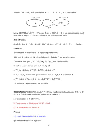
EJEMPLO 1. Sea 𝑇1:𝑅2 → 𝑅3 tal que 𝑇1(𝑥;𝑦) = (𝑥;𝑥 − 𝑦; 𝑦) y sea 𝑇2:𝑅3 → 𝑅2 tal que
𝑇2(𝑥; 𝑦;𝑧) = (𝑥 + 𝑧;𝑦).
a) Hallar si es posible 𝑇2o 𝑇1
b) Aplique 𝑇2o 𝑇1 al vector 𝑢 = (3;1)
c) Aplique 𝑇2o 𝑇1 al subespacio vectorial 𝑆 = {(𝑎; 𝑏) ∈ 𝑅2 𝑏 = 2𝑎
⁄ }
d) Hallar sus matrices asociadas a 𝑇1 , 𝑇2 y 𝑇2𝑜𝑇1
Solución.
a) La transformación lineal composición 𝑇2o 𝑇1 si es posible como se ve en seguida:
Siendo: 𝑇1(𝑥; 𝑦) = (𝑥;𝑥 − 𝑦; 𝑦) ; 𝑇2(𝑥;𝑦;𝑧) = (𝑥 + 𝑧;𝑦)
(𝑅2;𝑅; +; ∙) (𝑅3;𝑅; +; ∙) (𝑅2;𝑅; +; ∙)
𝑢 . 𝑇1(𝑢) . . 𝑇2[𝑇1(𝑢)] = (𝑇2o 𝑇1)(𝑢)
𝑇2o 𝑇1
𝑇2
𝑇1
>
>

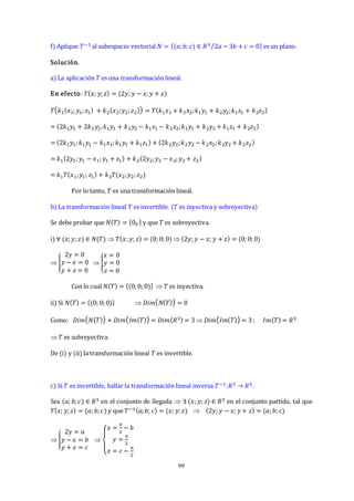
91
(𝑇2o 𝑇1)(𝑥;𝑦) = 𝑇2[𝑇1(𝑥; 𝑦)] = 𝑇2[(𝑥;𝑥 − 𝑦;𝑦)] = (𝑥 + 𝑦; 𝑥 − 𝑦)
Por lo tanto, (𝑇2o 𝑇1)(𝑥;𝑦) = (𝑥 + 𝑦;𝑥 − 𝑦)
b) Apliquemos 𝑇2o 𝑇1 al vector 𝑢 = (3;1)
Siendo, (𝑇2o 𝑇1)(𝑥;𝑦) = (𝑥 + 𝑦;𝑥 − 𝑦)  (𝑇2o 𝑇1)(3; 1) = (4;2)
c) Apliquemos 𝑇2o 𝑇1 al subespacio vectorial 𝑆 = {(𝑎;𝑏) ∈ 𝑅2 𝑏 = 2𝑎
⁄ }
Si 𝑆 = {(𝑎;𝑏) ∈ 𝑅2 𝑏 = 2𝑎
⁄ }  𝑆 = {(𝑎;2𝑎) ∈ 𝑅2 𝑎 ∈ 𝑅
⁄ }, es una recta.
Si 𝑢 = (𝑎;𝑏) ∈ 𝑆, 𝑢 = (𝑎;2𝑎)  (𝑇2o 𝑇1)(𝑎;2𝑎) = (3𝑎; −𝑎) = 𝑎(3; −1)
 𝑇(𝑆) = {(3𝑎;−𝑎) ∈ 𝑅2 𝑎 ∈ 𝑅
⁄ } , también es una recta.
d) Obteniendo las matrices asociadas correspondientes respecto a las bases canónicas:
i) Para: 𝑇1 (𝑥:𝑦) = (𝑥; 𝑥 − 𝑦;𝑦) o 𝑇1 [
𝑥
𝑦] = [
𝑥
𝑥 − 𝑦
𝑦
] = [
𝑥 + 0𝑦
𝑥 − 𝑦
0𝑥 + 𝑦
] = [
1 0
1 −1
0 1
] [
𝑥
𝑦]
 Su matriz asociada es: 𝐴𝑇
1
= [
1 0
1 −1
0 1
]
3×2
ii) Para: 𝑇2(𝑥;𝑦; 𝑧) = (𝑥 + 𝑧; 𝑦) o 𝑇2 [
𝑥
𝑦
𝑧
] = [
𝑥 + 𝑧
𝑦 ] = [
𝑥 + 0𝑦 + 𝑧
0𝑥 + 𝑦 + 0𝑧
]=[
1 0 1
0 1 0
][
𝑥
𝑦
𝑧
]
2
= [
1 0 1
0 1 0
]
2×3
iii) Para la composición: (𝑇2o 𝑇1)(𝑥; 𝑦) = (𝑥 + 𝑦;𝑥 − 𝑦)
 (𝑇2o 𝑇1) [
𝑥
𝑦] = [
𝑥 + 𝑦
𝑥 − 𝑦] = [
1 1
1 −1
][
𝑥
𝑦]
2𝑜𝑇1
= [
1 1
1 −1
]
2×2
Otra forma de hallar 𝐴 de la transformación lineal composición es dada por el producto de
matrices asociadas de cada transformación lineal que forman la composición, según una
proposición anterior:

92
𝐴𝑇
2𝑜𝑇1
= 𝐴𝑇
2
𝐴𝑇1
= [
1 0 1
0 1 0
]
2×3
.[
1 0
1 −1
0 1
]
3×2
= [
1 1
1 −1
]
2×2
EJEMPLO 2.Sean𝑇1:𝑅2 → 𝑅3talque𝑇1 (𝑥;𝑦) = (𝑥;𝑥 − 𝑦;𝑦) y 𝑇2:𝑅3 → 𝑅2 talque 𝑇2(𝑥;𝑦; 𝑧) =
(𝑥 + 𝑧;𝑦).
a) Hallar si es posible 𝑇1o 𝑇2 ,
b) Hallar las matrices asociadas a 𝑇1 , 𝑇2 y de 𝑇1o 𝑇2 .
c) Aplique 𝑇1o 𝑇2 al vector 𝑢 = (3;−4; 2)
d) Aplique 𝑇1o 𝑇2 al subespacio vectorial 𝑆 = {(𝑥;𝑦; 𝑧) ∈ 𝑅3 (𝑥;𝑦; 𝑧) = 𝑡(3; 2;1), 𝑡 ∈ 𝑅
⁄ }
Solución.
a) La transformación lineal composición 𝑇1 o 𝑇2 si es posible como se ve en seguida:
Siendo, 𝑇1(𝑥; 𝑦) = (𝑥;𝑥 − 𝑦; 𝑦) ; 𝑇2(𝑥;𝑦;𝑧) = (𝑥 + 𝑧;𝑦)
(𝑇1o 𝑇2)(𝑥;𝑦;𝑧) = 𝑇1[𝑇2(𝑥;𝑦;𝑧)] = 𝑇1[(𝑥 + 𝑧;𝑦)] = (𝑥 + 𝑧; 𝑥 + 𝑧 − 𝑦;𝑦)
Por lo tanto, (𝑇1o 𝑇2)(𝑥;𝑦;𝑧) = (𝑥 + 𝑧;𝑥 + 𝑧 − 𝑦; 𝑦)
b) Obteniendo las matrices asociadas correspondientes:
i) Para: 𝑇1 (𝑥:𝑦) = (𝑥; 𝑥 − 𝑦;𝑦) o 𝑇1 [
𝑥
𝑦] = [
𝑥
𝑥 − 𝑦
𝑦
] = [
𝑥 + 0𝑦
𝑥 − 𝑦
0𝑥 + 𝑦
] = [
1 0
1 −1
0 1
] [
𝑥
𝑦]
1
= [
1 0
1 −1
0 1
]
3×2
ii) Para: 𝑇2(𝑥;𝑦; 𝑧) = (𝑥 + 𝑧; 𝑦) o 𝑇2 [
𝑥
𝑦
𝑧
] = [
𝑥 + 𝑧
𝑦 ] = [
𝑥 + 0𝑦 + 𝑧
0𝑥 + 𝑦 + 0𝑧
] =
[
1 0 1
0 1 0
] [
𝑥
𝑦
𝑧
]
2
= [
1 0 1
0 1 0
]
2×3
iii) Para: (𝑇1o 𝑇2)(𝑥; 𝑦;𝑧) = (𝑥 + 𝑧; 𝑥 + 𝑧 − 𝑦;𝑦)

93
o (𝑇1o 𝑇2) [
𝑥
𝑦
𝑧
] = [
𝑥 + 𝑧
𝑥 + 𝑧 − 𝑦
𝑦
] = [
𝑥 + 0𝑦 + 𝑧
𝑥 − 𝑦 + 𝑧
0𝑥 + 𝑦 + 0𝑧
] = [
1 0 1
1 −1 1
0 1 0
][
𝑥
𝑦
𝑧
]
1𝑜𝑇2
= [
1 0 1
1 −1 1
0 1 0
]
3×3
Otraforma dehallar la matriz asociada de𝑇1𝑜𝑇2 , es dada porel productode matrices asociadas
de las transformaciones lineales, usando una proposición anterior:
𝐴𝑇
1𝑜𝑇2
= 𝐴𝑇
1
𝐴𝑇2
= [
1 0
1 −1
0 1
]
3×2
.[
1 0 1
0 1 0
]
2×3
= [
1 0 1
1 −1 1
0 1 0
]
3×3
c) Aplicando 𝑇1o 𝑇2 al vector 𝑢 = (3; −4;2)
Aplicando (𝑇1 o 𝑇2)(𝑥; 𝑦;𝑧) = (𝑥 + 𝑧; 𝑥 + 𝑧 − 𝑦;𝑦) al vector 𝑢 = (3; −4;2)
(𝑇1o 𝑇2)(3;−4; 2) =(5; 9;−4)
d) Aplicando 𝑇1o 𝑇2 al subespacio vectorial 𝑆 = {(𝑥;𝑦;𝑧) ∈ 𝑅3 (𝑥;𝑦;𝑧) = 𝑡(3;2; 1),𝑡 ∈ 𝑅
⁄ }
Aplicando (𝑇1o 𝑇2)(𝑥; 𝑦;𝑧) = (𝑥 + 𝑧; 𝑥 + 𝑧 − 𝑦;𝑦) al subespacio vectorial 𝑆 =
{(𝑥;𝑦;𝑧) ∈ 𝑅3 (𝑥;𝑦;𝑧) = 𝑡(3;2; 1),𝑡 ∈ 𝑅
⁄ }, es una recta.
Si 𝑢 = (3𝑡;2𝑡; 𝑡) ∈ 𝑆  (𝑇1 o 𝑇2)(3𝑡; 2𝑡;𝑡) = (4𝑡;2𝑡; 2𝑡) = 𝑡(4;2;2)
 𝑇(𝑆) = {(𝑥;𝑦;𝑧) ∈ 𝑅3 (𝑥;𝑦;𝑧) = 𝑡(4;2; 2),𝑡 ∈ 𝑅
⁄ }
Que también es un subespacio vectorial (una recta)
EJEMPLO 3. Sean 𝑇1:𝑅3 → 𝑅 tal que 𝑇1(𝑥;𝑦;𝑧) = 𝑥 − 𝑦 + 𝑧, y 𝑇2:𝑅 → 𝑅2 tal que 𝑇2(𝑥) =
(𝑥; −2𝑥).
a) Hallar 𝑇2o 𝑇1
b) Hallar las matrices asociadas
c) ¿Es posible hallar 𝑇1 o 𝑇2? Justifique su respuesta.
Solución.
a) La transformación lineal composición 𝑇2o 𝑇1 es posible como se ve en seguida:
(𝑇2o 𝑇1)(𝑥;𝑦;𝑧) =𝑇2[𝑇1(𝑥;𝑦;𝑧)] =𝑇2[(𝑥 − 𝑦 + 𝑧)] = (𝑥 − 𝑦 + 𝑧; −2𝑥 + 2𝑦 − 2𝑧)
Por lo tanto, (𝑇2o 𝑇1)(𝑥;𝑦;𝑧) = (𝑥 − 𝑦 + 𝑧; −2𝑥 + 2𝑦 − 2𝑧)

94
b) Obteniendo las matrices asociadas correspondientes:
i) Para: 𝑇1 (𝑥;𝑦;𝑧) = 𝑥 − 𝑦 + 𝑧 o 𝑇1 [
𝑥
𝑦
𝑧
] = [𝑥 − 𝑦 + 𝑧] = [1 −1 1] [
𝑥
𝑦
𝑧
]
1
= [1 −1 1]1×3
ii) Para: 𝑇2(𝑥) = (𝑥;−2𝑥) o 𝑇2[𝑥] = [
𝑥
−2𝑥
] = [
1
−2
] [𝑥]
2
= [
1
−2
]
2×1
iii) Para: (𝑇2o 𝑇1)(𝑥; 𝑦;𝑧) = (𝑥 − 𝑦 + 𝑧; −2𝑥 + 2𝑦 − 2𝑧)
O también: (𝑇2o 𝑇1) [
𝑥
𝑦
𝑧
] = [
𝑥 − 𝑦 + 𝑧
−2𝑥 + 2𝑦 − 2𝑧
] = [
1 −1 1
−2 2 −2
] [
𝑥
𝑦
𝑧
]
2o 𝑇1
= [
1 −1 1
−2 2 −2
]
2×3
Otra forma de hallar la matriz asociada es como el producto de las transformaciones lineales:
𝐴𝑇
2o 𝑇1
= 𝐴𝑇
2
𝐴𝑇1
= [
1
−2
]
2×1
[1 −1 1]1×3 = [
1 −1 1
−2 2 −2
]
2×3
c) La composición 𝑇1o 𝑇2 no es posible. ¿Por qué?
Sean 𝑇1:𝑅3 → 𝑅 tal que 𝑇1(𝑥;𝑦; 𝑧) = 𝑥 − 𝑦 + 𝑧, y 𝑇2: 𝑅 → 𝑅2 tal que 𝑇2(𝑥) = (𝑥; −2𝑥). ¿Es
posible hallar 𝑇1o 𝑇2?
No es posible, porque la dimensión de llegada de 𝑇1 es diferente de la dimensión del espacio de
partida de 𝑇2.
Probando esto: (𝑇1o 𝑇2)(𝑥) = 𝑇1[𝑇2(𝑥)] = 𝑇1(𝑥;−2𝑥), ¡aquí no es posible aplicar 𝑇1 dado que
esta aplica a vectores de tres componentes!
EJEMPLO 4. Sean 𝑇1:𝑅3 → 𝑃≤1 tal que 𝑇1(𝑎;𝑏;𝑐) = 𝑎 + (𝑏 + 𝑐)𝑥, y 𝑇2:𝑃≤1 → 𝑀2×2 tal que
𝑇2(𝑚 + 𝑛𝑥) = [
𝑚 𝑚 + 𝑛
𝑚 − 𝑛 𝑛
]
a) Hallar 𝑇2o 𝑇1
b) Hallar las matrices asociadas, respecto a las bases canónicas.

95
Solución.
a) Hallando: 𝑇2o 𝑇1
(𝑇2o 𝑇1) = 𝑇2[𝑇1(𝑎; 𝑏;𝑐)] = 𝑇2[𝑎 + (𝑏 + 𝑐)𝑥] = [
𝑎 𝑎 + 𝑏 + 𝑐
𝑎 − 𝑏 − 𝑐 𝑏 + 𝑐
]
Por lo tanto, (𝑇2o 𝑇1) =[
𝑎 𝑎 + 𝑏 + 𝑐
𝑎 − 𝑏 − 𝑐 𝑏 + 𝑐
]
b) Hallar las matrices asociadas, respecto a las bases canónicas.
Base de 𝑅3, [𝑣] = {(1;0; 0);(0; 1;0); (0;0;1)}, de 𝑃≤1 es [𝑤] = {1;𝑥} y de 𝑀2×2 es [𝑤] =
{[
1 0
0 0
] , [
0 1
0 0
] ,[
0 0
1 0
], [
0 0
0 1
]}
i) Siendo: 𝑇1:𝑅3 → 𝑃≤1 tal que 𝑇1(𝑎; 𝑏;𝑐) = 𝑎 + (𝑏 + 𝑐)𝑥 o 𝑇1 [
𝑎
𝑏
𝑐
] = 𝑎 + (𝑏 + 𝑐)𝑥
La matriz asociada es de la forma: 𝐴𝑇1
= [
𝑎11 𝑎12 𝑎13
𝑎21 𝑎22 𝑎23
]
2×3
𝑇1 [
1
0
0
]= 1 + 0𝑥 = 𝑎11(1) + 𝑎21(𝑥)= 1(1) + 0(𝑥)  𝑇1 [
1
0
0
]
[𝑤]
= [
1
0
]
𝑇1 [
0
1
0
]= 0 + 𝑥 = 𝑎12(1) + 𝑎22(𝑥)= 0(1) + 1(𝑥)  𝑇1 [
0
1
0
]
[𝑤]
= [
0
1
]
𝑇1 [
0
0
1
]= 0 + 𝑥 = 𝑎13(1) + 𝑎23(𝑥)= 0(1) + 1(𝑥)  𝑇1 [
0
0
1
]
[𝑤]
= [
0
1
]
Por lo tanto, la matriz asociada a 𝑇1 es: 𝐴𝑇
1
= [
1 0 0
0 1 1
]
3×2
ii) Siendo: 𝑇2:𝑃≤1 → 𝑀2×2 tal que 𝑇2(𝑚 + 𝑛𝑥) = [
𝑚 𝑚 + 𝑛
𝑚 − 𝑛 𝑛
] ; [𝑤] = {1;𝑥}
La matriz asociada es de la forma: 𝐴𝑇2
= [
𝑎11 𝑎12
𝑎21 𝑎22
𝑎13 𝑎14
𝑎23 𝑎24
]
4×2
𝑇2(1) =[
1 1
1 0
] = 𝑐1 [
1 0
0 0
] + 𝑐2[
0 1
0 0
] + 𝑐3 [
0 0
1 0
] + 𝑐4 [
0 0
0 1
]

96
 𝑇2(1) =[
1 1
1 0
] = 1 [
1 0
0 0
] + 1[
0 1
0 0
] + 1 [
0 0
1 0
] + 0 [
0 0
0 1
]  𝑇2(1)[𝑢] = [
1
1
1
0
]
𝑇2(1) =[
1 1
1 0
] = 𝑐1 [
1 0
0 0
] + 𝑐2[
0 1
0 0
] + 𝑐3 [
0 0
1 0
] + 𝑐4 [
0 0
0 1
]
 𝑇2(𝑥) =[
0 1
−1 1
] = 0 [
1 0
0 0
] + 1[
0 1
0 0
] + (−1)[
0 0
1 0
] + 1 [
0 0
0 1
]  𝑇2(1)[𝑢] = [
0
1
−1
1
]
Por lo tanto, la matriz asociada a 𝑇2 es: 𝐴𝑇
2
= [
1 0
1 1
1 −1
0 1
]
4×2
iii) La matriz asociada de la composición: 𝑇2𝑜𝑇1: 𝑅3 → 𝑀2×2
(𝑇2o 𝑇1) = 𝑇2[𝑇1(𝑎;𝑏; 𝑐)] = 𝑇2[𝑎 + (𝑏 + 𝑐)𝑥] = [
𝑎 𝑎 + 𝑏 + 𝑐
𝑎 − 𝑏 − 𝑐 𝑏 + 𝑐
]
Usando la proposiciónes:𝐴𝑇
2𝑜𝑇1
= 𝐴𝑇
2
𝐴𝑇
1
=[
1 0
1 1
1 −1
0 1
]
4×2
[
1 0 0
0 1 1
]
2×3
=[
1
1
0
1
0
1
1
0
−1
1
−1
1
]
4×3
Por lo tanto, la matriz asociada a 𝑇2𝑜𝑇1 es: 𝐴𝑇
2𝑜𝑇1
= [
1
1
0
1
0
1
1
0
−1
1
−1
1
]
4×3
No es posible, porque la dimensión de llegada de 𝑇1 , es 𝑛 = 2, es diferente de la dimensión del
espacio de partida de 𝑇2 , 𝑚 = 4.
Probando esto: (𝑇1o 𝑇2)(𝑚 + 𝑛𝑥) = 𝑇1[𝑇2(𝑚 + 𝑛𝑥)] = 𝑇1 [
𝑚 𝑚 + 𝑛
𝑚 − 𝑛 𝑛
],
¡Aquí no es posible aplicar 𝑇1 dado que esta aplica a vectores de la forma (𝑎;𝑏; 𝑐) ∈ 𝑅3!
3.4 TRANSFORMACIONES LINEALES INVERTIBLES.
DEFINICIÓN. Una transformación lineal 𝑇:𝑉 → 𝑊 siendo (𝑉;𝐾,+; ∙), (𝑊;𝐾,+; ∙) es invertible
si existe una aplicación𝐹:𝑊 → 𝑉 tal que la composición𝑇o 𝐹 = 𝐼𝑊 y la composición 𝐹𝑜𝑇 = 𝐼𝑉.
Asumiendo que 𝐹 es la inversa, se tiene 𝐹 = 𝑇−1 entonces 𝑇o𝐹 = 𝑇𝑜𝑇−1 = 𝐼𝑊 es la aplicación
identidad en 𝑊 y 𝐹o𝑇 = 𝑇−1𝑜𝑇 = 𝐼𝑉 es la aplicación identidad en 𝑉 .
OBSERVACIÓN. Si la transformación lineal es invertible, entonces la inversa es única y en
adelante se denotará por 𝑇−1.

97
Además: 𝑇o 𝑇−1 = 𝐼𝑊 es la identidad en 𝑊 ; y, 𝑇−1o T = 𝐼𝑉 es la identidad en 𝑉.
LEMA(PROPIEDAD).Si𝑇:𝑉 → 𝑊,siendo (𝑉;𝐾;+; ∙), (𝑊;𝐾;+; ∙), es una transformación lineal
invertible, su inversa 𝑇−1:𝑊 → 𝑉 también es una transformación lineal.
Demostración.
Siendo 𝑘1; 𝑘2 ∈ 𝐾 y 𝑌1; 𝑌2 ∈ 𝑊  𝑇−1(𝑘1𝑌
1 + 𝑘2𝑌
2) = 𝑘1𝑇−1(𝑌
1)+ 𝑘2𝑇−1(𝑌2) ¡Probar!
En efecto:
Recordar: Si 𝑇 es invertible  𝑇 es inyectiva y sobreyectiva.
Si 𝑌1; 𝑌2 ∈ 𝑊  ∃ 𝑋1; 𝑋2 ∈ 𝑉 tal que 𝑇(𝑋1) = 𝑌1y 𝑇(𝑋2) = 𝑌2por ser sobreyectiva
También se tiene que: 𝑋1 = 𝑇−1(𝑌
1)y 𝑋2 = 𝑇−1(𝑌
2), pues 𝑇 es invertible.
Como 𝑉 es un espacio vectorial: 𝑘1𝑋1 + 𝑘2𝑋2 ∈ 𝑉
 𝑇(𝑘1𝑋1 + 𝑘2𝑋2) = 𝑘1𝑇(𝑋1) + 𝑘2𝑇(𝑋2)= 𝑘1𝑌1 + 𝑘2𝑌2
 𝑘1𝑋1 + 𝑘2𝑋2 es único en 𝑉 que es aplicado en 𝑘1𝑌
1 + 𝑘2𝑌2 ∈ 𝑊 es único en 𝑊.
 𝑇−1(𝑘1𝑌
1 + 𝑘2𝑌
2)= 𝑘1𝑋1 + 𝑘2𝑋2 = 𝑘1𝑇−1(𝑌
1)+ 𝑘2𝑇−1(𝑌
2)
Por lo tanto, 𝑇−1 es una transformación lineal.
OBSERVACIÓN(PROPIEDAD).Siendo𝑇:𝑉 → 𝑊 una transformación lineal, siendo (𝑉;𝐾,+; ∙)y
(𝑊;𝐾,+; ∙) espacios vectoriales. En general, sea 𝑇 ∈ 𝐿(𝑉;𝑊).
a) 𝑇 es invertible  𝑇 es biyectiva.
b) 𝑇 es inyectiva  El núcleo de 𝑇, 𝑁(𝑇) = {0𝑉}
c) 𝑇 es sobreyectiva  𝑇(𝑉) = 𝑊
Prueba.
a1) () Si 𝑇 es invertible  𝑇 es biyectiva.
i) Si 𝑇 es invertible  𝑇 es inyectiva.
𝑇
(𝑉; 𝐾, +; ∙) (𝑊;𝐾,+; ∙)
𝑋 . . 𝑇(𝑋)
>
<
𝑇−1

98
Sean 𝑣𝑖;𝑣𝑗 ∈ 𝑉 y suponga que 𝑇(𝑣𝑖) = 𝑇(𝑣𝑗)  𝑇−1[𝑇(𝑣𝑖)] = 𝑇−1[𝑇(𝑣𝑗)]
 (𝑇−1𝑜𝑇)(𝑣𝑖) = (𝑇−1𝑜𝑇)(𝑣𝑗)  𝑣𝑖 = 𝑣𝑗
Por lo tanto, 𝑇 es inyectiva.
ii) Si 𝑇 es invertible  𝑇 es sobreyectiva.
Sea 𝑇 ∈ 𝐿(𝑉;𝑊). ∀ 𝑤 ∈ 𝑊, ∃ 𝑣 ∈ 𝑉 tal que 𝑇(𝑣) = 𝑤
Como 𝑇 es invertible ∀ 𝑤 ∈ 𝑊, ∃ 𝑣 ∈ 𝑉 tal que 𝑇−1(𝑤) = 𝑣  𝑇[𝑇−1(𝑤)] = 𝑇(𝑣) 𝑇(𝑣) = 𝑤
Por lo tanto, 𝑇 es sobreyectiva.
a2) () Si 𝑇 es biyectiva  𝑇 es invertible.
Se debe probar que: ∃ 𝑇−1:𝑊 → 𝑉 tal que 𝑇−1𝑜𝑇 = 𝐼𝑑𝑉  𝑇𝑜𝑇−1 = 𝐼𝑑𝑊
Por definición de 𝑇, ∀ 𝑣 ∈ 𝑉  𝑇(𝑣) = 𝑤 ∈ 𝑊 (1)
Por ser 𝑇 sobreyectiva, ∀ 𝑤 ∈ 𝑊, ∃ 𝑣 ∈ 𝑉 tal que 𝑇
̅(𝑤) = 𝑣 (2)
Por ser 𝑇 inyetiva el 𝑣 es único. Si 𝑇(𝑢) = 𝑇(𝑣)  𝑢 = 𝑣
De (1), 𝑇(𝑣) = 𝑤
 𝑇
̅[𝑇(𝑣)] = 𝑇
̅(𝑤)  𝑇
̅[𝑇(𝑣)] = 𝑣  (𝑇
̅𝑜𝑇)(𝑣) = 𝑣  𝑇
̅𝑜𝑇 = 𝐼𝑑𝑉 (3)
De (2), 𝑇
̅(𝑤) = 𝑣
 𝑇[𝑇
̅(𝑤)] = 𝑇(𝑣)  𝑇[𝑇
̅(𝑤)] = 𝑤  (𝑇𝑜𝑇
̅)(𝑤) = 𝑤  𝑇𝑜𝑇
̅ = 𝐼𝑑𝑊 (4)
Es decir 𝑇
̅ = 𝑇−1 es la inversa de 𝑇.
Por lo tanto, 𝑇 es invertible.
EJEMPLO 1. Sea la aplicación 𝑇: 𝑅3 → 𝑅3 tal que 𝑇(𝑥;𝑦; 𝑧) = (2𝑦;𝑦 − 𝑥; 𝑦 + 𝑧). Verificar las
afirmaciones que se dan:
a) La aplicación 𝑇 es una transformación lineal.
b) La transformación lineal 𝑇 es invertible.
c) Si 𝑇 es invertible, hallar la transformación lineal inversa 𝑇−1:𝑅3 → 𝑅3.
d) Compruebe que: 𝑇−1o 𝑇 = 𝐼𝑅3.
e) Aplique 𝑇 al subespacio vectorial 𝑆 = {(𝑥;𝑦,𝑧) ∈ 𝑅3 (𝑥;𝑦;𝑧) = 𝑡(1;2;3)
⁄ ,𝑡 ∈ 𝑅} es una
recta.

99
f) Aplique 𝑇−1 al subespacio vectorial 𝑁 = {(𝑎;𝑏; 𝑐) ∈ 𝑅3 2𝑎 − 3𝑏 + 𝑐 = 0
⁄ } es un plano.
Solución.
a) La aplicación 𝑇 es una transformación lineal.
En efecto: 𝑇(𝑥; 𝑦;𝑧) = (2𝑦;𝑦 − 𝑥;𝑦 + 𝑧)
𝑇 𝑘1(𝑥1;𝑦1;𝑧1) + 𝑘2(𝑥2;𝑦2;𝑧2) = 𝑇(𝑘1𝑥1 + 𝑘2𝑥2;𝑘1𝑦1 + 𝑘2𝑦2;𝑘1𝑧1 + 𝑘2𝑧2)
= (2𝑘1𝑦1 + 2𝑘2𝑦2;𝑘1𝑦1 + 𝑘2𝑦2 − 𝑘1𝑥1 − 𝑘2𝑥2;𝑘1𝑦1 + 𝑘2𝑦2 + 𝑘1𝑧1 + 𝑘2𝑧2)
= (2𝑘1𝑦1;𝑘1𝑦1 − 𝑘1𝑥1;𝑘1𝑦1 + 𝑘1𝑧1) + (2𝑘2𝑦2;𝑘2𝑦2 − 𝑘2𝑥2;𝑘2𝑦2 + 𝑘2𝑧2)
= 𝑘1(2𝑦1;𝑦1 − 𝑥1;𝑦1 + 𝑧1) + 𝑘2(2𝑦2;𝑦2 − 𝑥2;𝑦2 + 𝑧2)
= 𝑘1𝑇(𝑥1;𝑦1; 𝑧1) + 𝑘2𝑇(𝑥2;𝑦2;𝑧2)
Por lo tanto, 𝑇 es una transformación lineal.
b) La transformación lineal 𝑇 es invertible. (𝑇 es inyectiva y sobreyectiva)
Se debe probar que 𝑁(𝑇) = {0𝑉} y que 𝑇 es sobreyectiva.
i) ∀ (𝑥;𝑦;𝑧) ∈ 𝑁(𝑇)  𝑇(𝑥;𝑦; 𝑧) = (0; 0;0)  (2𝑦;𝑦 − 𝑥; 𝑦 + 𝑧) = (0; 0;0)
 {
2𝑦 = 0
𝑦 − 𝑥 = 0
𝑦 + 𝑧 = 0
 {
𝑥 = 0
𝑦 = 0
𝑧 = 0
Con lo cual 𝑁(𝑇) = {(0;0; 0)}  𝑇 es inyectiva.
ii) Si 𝑁(𝑇) = {(0; 0;0)}  𝐷𝑖𝑚 𝑁(𝑇) = 0
Como: 𝐷𝑖𝑚 𝑁(𝑇) + 𝐷𝑖𝑚 𝐼𝑚(𝑇) = 𝐷𝑖𝑚(𝑅3) = 3  𝐷𝑖𝑚 𝐼𝑚(𝑇) = 3 ; 𝐼𝑚(𝑇) = 𝑅3
 𝑇 es sobreyectiva.
De (i) y (ii) la transformación lineal 𝑇 es invertible.
c) Si 𝑇 es invertible, hallar la transformación lineal inversa 𝑇−1:𝑅3 → 𝑅3.
Sea (𝑎; 𝑏;𝑐) ∈ 𝑅3 en el conjunto de llegada  ∃ (𝑥;𝑦; 𝑧) ∈ 𝑅3 en el conjunto partida, tal que
𝑇(𝑥; 𝑦;𝑧) = (𝑎;𝑏;𝑐) y que 𝑇−1(𝑎;𝑏; 𝑐) = (𝑥; 𝑦:𝑧)  (2𝑦;𝑦 − 𝑥; 𝑦 + 𝑧) = (𝑎;𝑏; 𝑐)
 {
2𝑦 = 𝑎
𝑦 − 𝑥 = 𝑏
𝑦 + 𝑧 = 𝑐

{
𝑥 =
𝑎
2
− 𝑏
𝑦 =
𝑎
2
𝑧 = 𝑐 −
𝑎
2

100
Por lo tanto, la transformación lineal inversa será: 𝑇−1(𝑎;𝑏; 𝑐) = (
𝑎
2
− 𝑏;
𝑎
2
;𝑐 −
𝑎
2
)
d) Compruebe que: 𝑇−1o 𝑇 = 𝐼𝑅3. También 𝑇𝑜𝑇−1 = 𝐼𝑅3
En efecto: (𝑇−1o 𝑇)(𝑥;𝑦; 𝑧) = 𝑇−1[𝑇(𝑥;𝑦;𝑧)] = 𝑇−1(2𝑦;𝑦 − 𝑥;𝑦 + 𝑧)
= (
2𝑦
2
− 𝑦 + 𝑥;
2𝑦
2
;𝑦 + 𝑧 −
2𝑦
2
)  (𝑇−1o𝑇)(𝑥;𝑦;𝑧) = (𝑥;𝑦,𝑧) = 𝐼𝑅3
Por lo tanto: (𝑇−1o𝑇) = 𝐼𝑅3
e) Aplique 𝑇 al subespacio vectorial 𝑆 = {(𝑥;𝑦,𝑧) ∈ 𝑅3 (𝑥;𝑦;𝑧) = 𝑡(1;2;3)
⁄ ,𝑡 ∈ 𝑅} es una
recta.
𝑇(𝑥; 𝑦;𝑧) = 𝑇(𝑡; 2𝑡;3𝑡) = (2(2𝑡);2𝑡 − 𝑡;2𝑡 + 3𝑡) = (4𝑡;𝑡; 5𝑡) = 𝑡(4;1; 5)
En el espacio de llegada 𝑇(𝑆) = {(𝑥;𝑦, 𝑧) ∈ 𝑅3 (𝑥;𝑦; 𝑧) = 𝑡(4; 1;5)
⁄ ,𝑡 ∈ 𝑅}es una recta.
f) Aplique 𝑇−1 al subespacio vectorial 𝑁 = {(𝑎;𝑏; 𝑐) ∈ 𝑅3 2𝑎 − 3𝑏 + 𝑐 = 0
⁄ } es un plano.
𝑇−1(𝑎;𝑏; 𝑐) = 𝑇−1(𝑎;𝑏; 3𝑏 − 2𝑎) = (
𝑎
2
− 𝑏;
𝑎
2
; 3𝑏 − 2𝑎 −
𝑎
2
) = (
𝑎
2
− 𝑏;
𝑎
2
;3𝑏 −
5𝑎
2
) = (𝑥;𝑦; 𝑧)
En el conjunto de llegada (
𝑎
2
− 𝑏;
𝑎
2
;3𝑏 −
5𝑎
2
) = (𝑥;𝑦;𝑧) 
{
𝑎
2
− 𝑏 = 𝑥
𝑎
2
= 𝑦
3𝑏 −
5𝑎
2
= 𝑧
 {
𝑥 − 𝑦 = −𝑏
𝑧 = 3𝑏 −
5𝑎
2
 𝑧 = −3𝑥 − 2𝑦; es la ecuación de un plano.
En el espacio de llegada 𝑇−1(𝑁) = {(𝑥;𝑦; 𝑧) ∈ 𝑅3 𝑧 = −3𝑥 − 2𝑦
⁄ }, también es un plano.
EJEMPLO 2. Sea la transformación lineal 𝑇: 𝑅2 → 𝑃≤1tal que 𝑇(𝑎; 𝑏) = 2𝑎 + (𝑎 + 𝑏)𝑥
a) Muestre que 𝑇 es una transformación lineal.
b) Muestre que 𝑇 es biyectiva.
c) Hallar la transformación lineal inversa de 𝑇.
d) Muestre que 𝑇−1:𝑃≤1 → 𝑅2 es una transformación lineal.
e) Hallar las matrices asociadas a la transformaciones lineales 𝑇 y 𝑇−1.

101
f) Halle la relación entre la matrices asociadas a las transformaciones lineales 𝑇 y 𝑇−1
Solución.
a) 𝑇 es una transformación lineal, pues 𝑇(𝑘𝑢 + 𝑣) = 𝑘𝑇(𝑢) + 𝑇(𝑣), ∀𝑢,𝑣 ∈ 𝑅2,∀𝑘 ∈ 𝑅
En efecto:
𝑇(𝑘𝑢 + 𝑣) = 𝑇 𝑘(𝑎;𝑏) + (𝑐;𝑑) = 𝑇(𝑘𝑎 + 𝑐; 𝑘𝑏 + 𝑑) = 2(𝑘𝑎 + 𝑐) + (𝑘𝑎 + 𝑐 + 𝑘𝑏 + 𝑑)𝑥
= 2𝑘𝑎 + 2𝑐 + 𝑘(𝑎 + 𝑏)𝑥 + (𝑐 + 𝑑)𝑥 = 2𝑘𝑎 + 𝑘(𝑎 + 𝑏)𝑥 + 2𝑐 + (𝑐 + 𝑑)𝑥
= 𝑘(2𝑎 + (𝑎 + 𝑏)𝑥) + (2𝑐 + (𝑐 + 𝑑)𝑥) = 𝑘𝑇(𝑎; 𝑏) + 𝑇(𝑐;𝑑) = 𝑘𝑇(𝑢) + 𝑇(𝑣)
b) 𝑇 es biyectiva.
b1) 𝑇 es inyectiva, pues 𝑇(𝑎;𝑏) = 𝑇(𝑐;𝑑)  2𝑎 + (𝑎 + 𝑏)𝑥 = 2𝑐 + (𝑐 + 𝑑)𝑥
 {
2𝑎 = 2𝑐
𝑎 + 𝑏 = 𝑐 + 𝑑
 {
𝑎 = 2
𝑏 = 𝑑
 (𝑎;𝑏) = (𝑐;𝑑)
b2) 𝑇 es sobreyectiva, pues ∀𝑚 + 𝑛𝑥 ∈ 𝑃≤1, existe (𝑎;𝑏) ∈ 𝑅2 tal que 𝑇(𝑎; 𝑏) = 𝑚 + 𝑛𝑥
𝑇(𝑎;𝑏) = 𝑚 + 𝑛𝑥  2𝑎 + (𝑎 + 𝑏)𝑥 = 𝑚 + 𝑛𝑥  {
2𝑎 = 𝑚
𝑎 + 𝑏 = 𝑛
 {
𝑎 =
𝑚
2
𝑏 = 𝑛 −
𝑚
2
 ∀𝑚 + 𝑛𝑥 ∈ 𝑃≤1, ∃(𝑎; 𝑏) = (
𝑚
2
;
2𝑛−𝑚
2
) tal que 𝑇(𝑎; 𝑏) = 𝑇 (
𝑚
2
;
2𝑛−𝑚
2
)
= 2 (
𝑚
2
) + (
𝑚
2
+
2𝑛−𝑚
2
)𝑥 = 𝑚 + 𝑛𝑥  𝑇 (
𝑚
2
;
2𝑛−𝑚
2
) = 𝑚 + 𝑛𝑥
c) Hallando la transformación lineal inversa de 𝑇. Es decir se debe hallar 𝑇−1:𝑃≤1 → 𝑅2
De la sobreyectividad 𝑇(
𝑚
2
;
2𝑛−𝑚
2
) = 𝑚 + 𝑛𝑥
Aplicando 𝑇−1 a ambos lados 𝑇−1(𝑚 + 𝑛𝑥) = (
𝑚
2
;
2𝑛−𝑚
2
)
d) 𝑇−1:𝑃≤1 → 𝑅2 es una transformación lineal.
En efecto:
𝑇−1 𝑘(𝑚 + 𝑛𝑥) + (𝑝 + 𝑞𝑥) = 𝑇(𝑘𝑚 + 𝑘𝑛𝑥 + 𝑝 + 𝑞𝑥) = 𝑇 (𝑘𝑚 + 𝑝) + (𝑘𝑛 + 𝑞)𝑥
= (
𝑘𝑚+𝑝
2
;
2(𝑘𝑛+𝑞)−(𝑘𝑚+𝑝)
2
)= (𝑘
𝑚
2
+
𝑝
2
;
2𝑘𝑛
2
+
2𝑞
2
− 𝑘
𝑚
2
−
𝑝
2
) = 𝑘 (
𝑚
2
;
2𝑘𝑛
2
−
𝑚
2
) + (
𝑝
2
+
2𝑞
2
−
𝑝
2
)
= 𝑘𝑇(𝑚 + 𝑛𝑥) + 𝑇(𝑝 + 𝑞𝑥)
e) Las matrices asociadas a las transformaciones lineales 𝑇 y 𝑇−1.

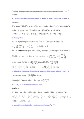
102
e1) Matriz asociada a la transformación lineal 𝑇(𝑎; 𝑏) = 2𝑎 + (𝑎 + 𝑏)𝑥
Bases canónicas: 𝐵𝑅2 = {(1;0),(0;1)} ; 𝐵𝑃≤1
= {1,𝑥}
La matriz será de la forma: 𝐴𝑇 = [
𝑎11 𝑎12
𝑎21 𝑎22
]
𝑇(1; 0) = 2 + 𝑥 = 𝑎11(1) + 𝑎21(𝑥) = 2(1) + 1(𝑥)
𝑇(0; 1) = 0 + 𝑥 = 𝑎12(1) + 𝑎22(𝑥) = 0(1) + 1(𝑥)
 𝐻 = [
𝑎11 𝑎21
𝑎12 𝑎22
]=[
2 0
1 1
]  𝐴𝑇 = 𝐻𝑡 = [
𝑎11 𝑎12
𝑎21 𝑎22
] = [
2 1
0 1
]  𝐴𝑇 = [
2 1
0 1
]
e2) Matriz asociada a la transformación lineal inversa: 𝑇−1(𝑚 + 𝑛𝑥) = (
𝑚
2
;
2𝑛−𝑚
2
)
La matriz será de la forma: 𝐴𝑇−1 = [
𝑏11 𝑏12
𝑏21 𝑏22
]
𝑇−1(1) = (
1
2
; −
1
2
) = 𝑏11(1;0) + 𝑏21(0;1) =
1
2
(1; 0) −
1
2
(0; 1)
𝑇−1(𝑥) = (0;1) = 𝑏12(1;0) + 𝑏22(0;1) = 0(1;0) + 1(0;1)
 𝐻 = [
𝑏11 𝑏21
𝑏12 𝑏22
]=[
1
2
0
−
1
2
1
]  𝐴𝑇−1 = 𝐻𝑡 = [
𝑏11 𝑏12
𝑏21 𝑏22
] = [
1
2
−
1
2
0 1
]  𝐴𝑇−1 = [
1
2
−
1
2
0 1
]
f) Hallando la inversa de la matriz asociada a la transformación lineal 𝑇.
f1) Multiplicándose las matrices asociadas halladas:
(𝐴𝑇)(𝐴𝑇−1) = [
2 1
0 1
] = [
1
2
−
1
2
0 1
] = [
2 (
1
2
) + 1(0) 2(−
1
2
) + 1(1)
0 (
1
2
) + 1(0) 0(−
1
2
) + 1(1)
] = [
1 0
0 1
] = 𝐼2×2
f2) Inversa para el caso de matrices de orden 2 × 2:
Si 𝐴𝑇 = [
𝑎11 𝑎12
𝑎21 𝑎22
]  𝐴𝑇
−1
=
1
𝐷𝑒𝑡(𝐴𝑇)
[
𝑎22 −𝑎12
𝑎21 𝑎11
]
Dado que 𝐴𝑇 = [
2 1
0 1
] 𝐷𝑒𝑡(𝐴𝑇) = 2
 𝐴𝑇
−1
=
1
𝐷𝑒𝑡(𝐴𝑇)
[
𝑎22 −𝑎12
−𝑎21 𝑎11
] =
1
2
[
1 −1
0 2
] = [
1
2
−
1
2
0 1
]
OBSERVACIÓN. Las matrices asociadas 𝐴𝑇 y 𝐴𝑇
−1
respectivamente a las transformaciones
lineales 𝑇 y su inversa 𝑇−1 es que una es inversa de la otra.

103
Profesor: Dionicio Milton Chávez Muñoz

3 capitulo-iii-matriz-asociada-sem-13-t-l-c

Recommended

Recommended

More Related Content

What's hot

What's hot (20)

Similar to 3 capitulo-iii-matriz-asociada-sem-13-t-l-c

Similar to 3 capitulo-iii-matriz-asociada-sem-13-t-l-c (20)

Recently uploaded

Recently uploaded (20)

3 capitulo-iii-matriz-asociada-sem-13-t-l-c