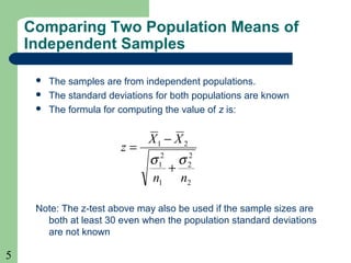
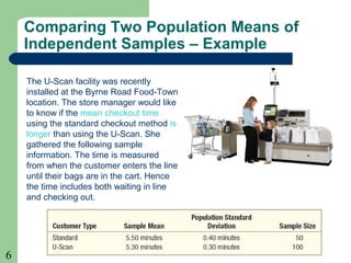
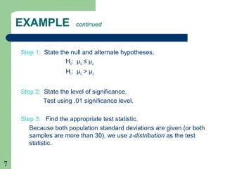
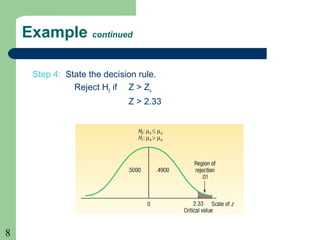
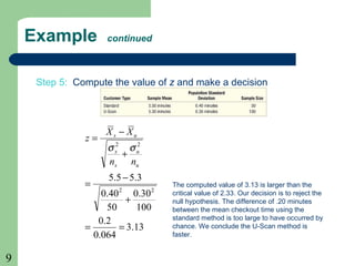
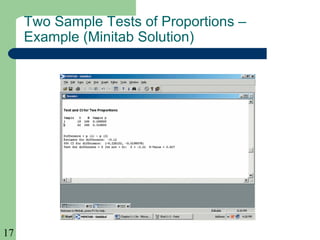
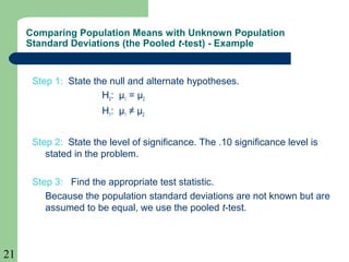
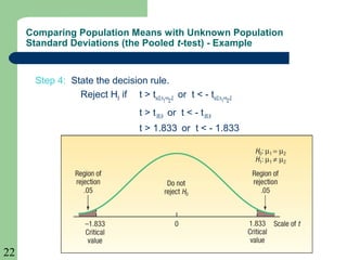
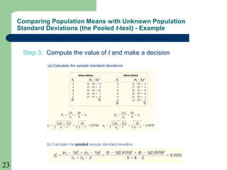
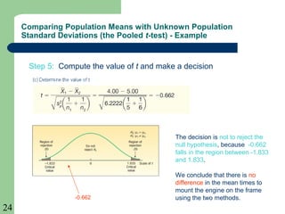
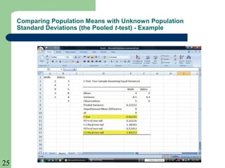
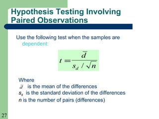
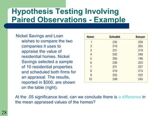
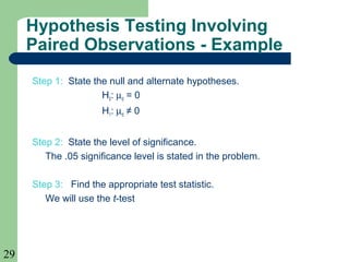
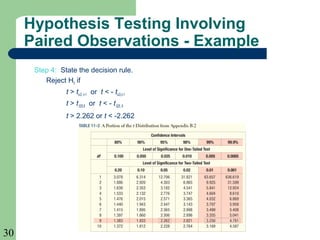
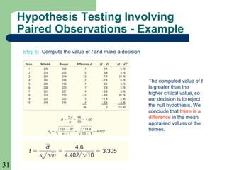
The document discusses different types of two-sample hypothesis tests, including tests comparing two population means of independent samples, two population proportions, and paired or dependent samples. It provides examples and step-by-step explanations of how to conduct two-sample t-tests, z-tests, and tests of proportions. Key points covered include determining the appropriate test statistic based on sample size and characteristics, stating the null and alternative hypotheses, test criteria, and decisions rules.

1. ©The McGraw-Hill Companies, Inc. 2008McGraw-Hill/Irwin
Two-sample Tests of Hypothesis
Chapter 11

2. 2
GOALS
1. Conduct a test of a hypothesis about the
difference between two independent
population means.
2. Conduct a test of a hypothesis about the
difference between two population proportions.
3. Conduct a test of a hypothesis about the mean
difference between paired or dependent
observations.
4. Understand the difference between dependent
and independent samples.

3. 3
Comparing two populations – Some
Examples
1. Is there a difference in the mean value of
residential real estate sold by male agents
and female agents in south Florida?
2. Is there a difference in the mean number of
defects produced on the day and the
afternoon shifts at Kimble Products?
3. Is there a difference in the mean number of
days absent between young workers (under
21 years of age) and older workers (more than
60 years of age) in the fast-food industry?

4. 4
Comparing two populations – Some
Examples (continued)
4. Is there is a difference in the proportion of
Ohio State University graduates and
University of Cincinnati graduates who
pass the state Certified Public Accountant
Examination on their first attempt?
5. Is there an increase in the production rate
if music is piped into the production area?

5. 5
Comparing Two Population Means of
Independent Samples
 The samples are from independent populations.
 The standard deviations for both populations are known
 The formula for computing the value of z is:
Note: The z-test above may also be used if the sample sizes are
both at least 30 even when the population standard deviations
are not known
2
2
2
1
2
1
21
nn
XX
z
σσ
+
−
=

6. 6
Comparing Two Population Means of
Independent Samples – Example
The U-Scan facility was recently
installed at the Byrne Road Food-Town
location. The store manager would like
to know if the mean checkout time
using the standard checkout method is
longer than using the U-Scan. She
gathered the following sample
information. The time is measured
from when the customer enters the line
until their bags are in the cart. Hence
the time includes both waiting in line
and checking out.

7. 7
EXAMPLE continued
Step 1: State the null and alternate hypotheses.
H0: µS ≤ µU
H1: µS > µU
Step 2: State the level of significance.
Test using .01 significance level.
Step 3: Find the appropriate test statistic.
Because both population standard deviations are given (or both
samples are more than 30), we use z-distribution as the test
statistic.

8. 8
Example continued
Step 4: State the decision rule.
Reject H0 if Z > Zα
Z > 2.33

9. 9
Example continued
Step 5: Compute the value of z and make a decision
13.3
064.0
2.0
100
30.0
50
40.0
3.55.5
22
22
==
+
−
=
+
−
=
u
u
s
s
us
nn
XX
z
σσ
The computed value of 3.13 is larger than the
critical value of 2.33. Our decision is to reject the
null hypothesis. The difference of .20 minutes
between the mean checkout time using the
standard method is too large to have occurred by
chance. We conclude the U-Scan method is
faster.

10. 10
Two-Sample Tests about Proportions
Here are several examples.
 The vice president of human resources wishes to know whether
there is a difference in the proportion of hourly employees who
miss more than 5 days of work per year at the Atlanta and the
Houston plants.
 General Motors is considering a new design for the Pontiac
Grand Am. The design is shown to a group of potential buyers
under 30 years of age and another group over 60 years of age.
Pontiac wishes to know whether there is a difference in the
proportion of the two groups who like the new design.
 A consultant to the airline industry is investigating the fear of
flying among adults. Specifically, the company wishes to know
whether there is a difference in the proportion of men versus
women who are fearful of flying.

11. 11
Two Sample Tests of Proportions
 We investigate whether two samples came from
populations with an equal proportion of successes.
 The two samples are pooled using the following
formula.

12. 12
Two Sample Tests of Proportions
continued
The value of the test statistic is computed from
the following formula.

13. 13
Manelli Perfume Company recently developed a new
fragrance that it plans to market under the name Heavenly. A
number of market studies indicate that Heavenly has very
good market potential. The Sales Department at Manelli is
particularly interested in whether there is a difference in the
proportions of younger and older women who would purchase
Heavenly if it were marketed.
Two independent populations, a population consisting of the
younger women and a population consisting of the older
women, were surveyed. Each sampled woman was asked to
smell Heavenly and indicate whether she likes the fragrance
well enough to purchase a bottle. Of 100 young women, 19
liked the Heavenly fragrance well enough to purchase
Similarly, a sample of 200 older women, 62 liked the
fragrance well enough to make a purchase.
Two Sample Tests of Proportions -
Example

14. 14
Step 1: State the null and alternate hypotheses.
H0: π1 = π2
H1: π1 ≠ π2
note: keyword “there is a difference in the proportion”
We designate π1 as the proportion of young women who would purchase
Heavenly and π2 as the proportion of older women who would purchase
Step 2: State the level of significance.
The .05 significance level is chosen.
Step 3: Find the appropriate test statistic.
We will use the z-distribution
Two Sample Tests of Proportions -
Example

15. 15
Step 4: State the decision rule.
Reject H0 if Z > Zα/2 or Z < - Zα/2
Z > 1.96 or Z < -1.96
Two Sample Tests of Proportions -
Example

16. 16
Step 5: Compute the value of z and make a decision
The computed value of -2.21 is in the area of rejection. Therefore, the null hypothesis is
rejected at the .05 significance level. To put it another way, we reject the null hypothesis
that the proportion of young women who would purchase Heavenly is equal to the
proportion of older women who would purchase Heavenly.
Two Sample Tests of Proportions -
Example

17. 17
Two Sample Tests of Proportions –
Example (Minitab Solution)

18. 18
Comparing Population Means with Unknown
Population Standard Deviations (the Pooled t-test)
The t distribution is used as the test statistic if one
or more of the samples have less than 30
observations. The required assumptions are:
1. Both populations must follow the normal
distribution.
2. The populations must have equal standard
deviations.
3. The samples are from independent populations.

19. 19
Small sample test of means continued
Finding the value of the test
statistic requires two
steps.
1. Pool the sample standard
deviations.
2. Use the pooled standard
deviation in the formula.
2
)1()1(
21
2
22
2
112
−+
−+−
=
nn
snsn
sp






+
−
=
21
2
21
11
nn
s
XX
t
p

20. 20
Owens Lawn Care, Inc., manufactures and assembles
lawnmowers that are shipped to dealers throughout the
United States and Canada. Two different procedures have
been proposed for mounting the engine on the frame of the
lawnmower. The question is: Is there a difference in the
mean time to mount the engines on the frames of the
lawnmowers? The first procedure was developed by longtime
Owens employee Herb Welles (designated as procedure 1),
and the other procedure was developed by Owens Vice
President of Engineering William Atkins (designated as
procedure 2). To evaluate the two methods, it was decided to
conduct a time and motion study.
A sample of five employees was timed using the Welles
method and six using the Atkins method. The results, in
minutes, are shown on the right.
Is there a difference in the mean mounting times? Use the .
10 significance level.
Comparing Population Means with Unknown
Population Standard Deviations (the Pooled t-test)

21. 21
Step 1: State the null and alternate hypotheses.
H0: µ1 = µ2
H1: µ1 ≠ µ2
Step 2: State the level of significance. The .10 significance level is
stated in the problem.
Step 3: Find the appropriate test statistic.
Because the population standard deviations are not known but are
assumed to be equal, we use the pooled t-test.
Comparing Population Means with Unknown Population
Standard Deviations (the Pooled t-test) - Example

22. 22
Step 4: State the decision rule.
Reject H0 if t > tα/2,n1+n2-2 or t < - tα/2,n1+n2-2
t > t.05,9 or t < - t.05,9
t > 1.833 or t < - 1.833
Comparing Population Means with Unknown Population
Standard Deviations (the Pooled t-test) - Example

23. 23
Step 5: Compute the value of t and make a decision
(a) Calculate the sample standard deviations
Comparing Population Means with Unknown Population
Standard Deviations (the Pooled t-test) - Example

24. 24
Step 5: Compute the value of t and make a decision
Comparing Population Means with Unknown Population
Standard Deviations (the Pooled t-test) - Example
-0.662
The decision is not to reject the
null hypothesis, because -0.662
falls in the region between -1.833
and 1.833.
We conclude that there is no
difference in the mean times to
mount the engine on the frame
using the two methods.

25. 25
Comparing Population Means with Unknown Population
Standard Deviations (the Pooled t-test) - Example

26. 26
Two-Sample Tests of Hypothesis:
Dependent Samples
Dependent samples are samples that are paired or
related in some fashion.
For example:
– If you wished to buy a car you would look at the
same car at two (or more) different dealerships
and compare the prices.
– If you wished to measure the effectiveness of a
new diet you would weigh the dieters at the start
and at the finish of the program.

27. 27
Hypothesis Testing Involving
Paired Observations
Use the following test when the samples are
dependent:
t
d
s nd
=
/
d
Where
is the mean of the differences
sd is the standard deviation of the differences
n is the number of pairs (differences)

28. 28
Nickel Savings and Loan
wishes to compare the two
companies it uses to
appraise the value of
residential homes. Nickel
Savings selected a sample
of 10 residential properties
and scheduled both firms for
an appraisal. The results,
reported in $000, are shown
on the table (right).
Hypothesis Testing Involving
Paired Observations - Example
At the .05 significance level, can we conclude there is a difference in
the mean appraised values of the homes?

29. 29
Step 1: State the null and alternate hypotheses.
H0: µd = 0
H1: µd ≠ 0
Step 2: State the level of significance.
The .05 significance level is stated in the problem.
Step 3: Find the appropriate test statistic.
We will use the t-test
Hypothesis Testing Involving
Paired Observations - Example

30. 30
Step 4: State the decision rule.
Reject H0 if
t > tα/2, n-1 or t < - tα/2,n-1
t > t.025,9 or t < - t.025, 9
t > 2.262 or t < -2.262
Hypothesis Testing Involving
Paired Observations - Example

31. 31
Step 5: Compute the value of t and make a decision
The computed value of t
is greater than the
higher critical value, so
our decision is to reject
the null hypothesis. We
conclude that there is a
difference in the mean
appraised values of the
homes.
Hypothesis Testing Involving
Paired Observations - Example

32. 32
Hypothesis Testing Involving Paired Observations –
Excel Example

33. 33
End of Chapter 11