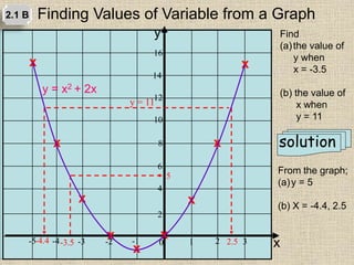
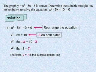
Here are the steps to solve this problem: 1) The given equation is: y = x2 + 2x 2) To complete the table, we need to calculate the value of y when x = -3 and when x = 1 3) When x = -3: y = (-3)2 + 2(-3) y = 9 - 6 y = 3 4) When x = 1: y = 12 + 2(1) y = 1 + 2 y = 3 So the completed table is: Table 1 x -3 1 y 3 3 (b) Sketch the graph of y = x2 + 2

4. CHAPTER 2
GRAPHS OF FUNCTIONS II
2.1 GRAPHS OF FUNCTIONS
• The graph of a function is a set of points on
the Cartesian Plane that satisfy the function
• Information is presented in the form of graphs
• Graph are widely used in science and technology
• Graphs are very useful to researchers, scientists
and economist

5. The different type of functions and respective power of x
Type of
function
General form Example Highest
power of variable x
Linear
Quadratic
Cubic
Reciprocal
y = ax + c
y = ax2 + bx + c
y = ax3 + bx2 + cx + d
y = a
x
y = 3x
y = -4x + 5
y = 2x2
y = -3x2 + 2x
y = 2x2 + 5x + 1
y = 2x3
y = -3x3 + 5x
y = 2x3 - 3x + 6
y = 4
x
y = - 2
x
1
3
-1
2
y = ax3
y = ax3 + bx
y = ax3 + bx + c
a ≠ 0

6. LINEAR FUNCTION

7. LINEAR FUNCTION

8. QUADRATIC FUNCTION

9. QUADRATIC FUNCTION

10. QUBIC FUNCTION

11. QUBIC FUNCTION

12. RECIPROCAL FUNCTION

13. RECIPROCAL FUNCTION

14. • Using calculator to complete the tables
• Using the scale given to mark the points
on the x-axis and y-axis
• Plotting all the points using the scale given

15. COMP

16. CALC Memory
Example 1
Calculate the result
for Y = 3X – 5,
when X = 4, and when X = 6
)3
X
- 5
CALC
3X – 5
4 = 7
CALC 6 = 13
ALPHA

17. CALC Memory
Example 2
Calculate the result
for Y = X2 + 3X – 12,
when X = 7, and when X = 8
) 3
X
x2
+
ALPHA
)
X
- 21
CALC
X2 + 3X – 12
7 = 58
CALC 8 = 76
ALPHA

18. CALC Memory
Example 3
Calculate the result
for Y = 2X2 + X – 6,
when X = 3, and when X = -3
)
3
X
x2
+
ALPHA
)
X
- 6
CALC
2X2 + X – 6
3 = 15
CALC (-) = 9
ALPHA
2

19. CALC Memory
Example 4
Calculate the result
for Y = -X3 + 2X + 5,
when X = 2, and when X = -1
)
1
X
x2
+ 2
ALPHA
)
X
+ 5
-X3 + 2X + 5 2 = 1
CALC (-) = 4
ALPHA
(-)
SHIFT x3
CALC

20. Example 5
Calculate the result
for Y = 6 when X = -3,
X
and when X = 0.5
)
XALPHA
3CALC (-) = -2
6
CALC 0 . 125 =
ab/c 6┘x

21. Example 6
Calculate the result
for Y = 6 when X = -3,
X
and when X = 0.5
)
XALPHA
3CALC (-) = -2
6
CALC 0 . 125 =
x-1
6x-1

22. Y = -2X2 + 40
X 0 0.5 1 1.5 2 3 3.5 4
Y
Y = X3 – 3X + 3
X -3 -2 -1 0 0.5 1 1.5 2
Y
Y = -16
X
X -4 -3 -2 -1 1 2 3 4
Y
40 39.5 38 35.5 32 22 15.5 8
-15 1 5 3 16.25 1.875 51
4 5.33 8 16 -16 -8 -5.33 -4

23. 2(4)2 + 5(4) – 1 = 51
Using Calculator
2 ( )4 x2 + 5 ( 4 )
- 1 =

24. (-2)3 - 12(-2) + 10 = 26
Using Calculator
2( ) x2
+ 1 0
(-) 1
=
SHIFT - 2
2( )(-)
2( ) 3
+ 1 0
(-) 1
=
V
- 2
2( )(-)
OR

25. Using Calculator
6
(-3)
= -2
3( )6 ÷ (-) =

26. x -5 -4 -3 -2 -1 0 1 2 3
y 15 8 0 -1 0 3 15
y = x2 + 2x
y = (
-3
)2
+ 2 (
-3
) = 3
y = (
2
)2
+ 2 (
2
) = 8
3
8

27. x -4 -2.5 -1 -0.5 0.5 1 2 3.2 4
y 1 1.6 8 -8 -4 -1.25 -1
4
2
y = -4
( )
=
y = -4
( )
=
-1
4 -2-2
y = -4
x
Completing the table of values
-1 2

28. 2.4 3.0 3.9
x-axis scale : 2 cm to 2 units
Marking the points on the x-axis and y-axis
2 4

29. -4 -2
-3.6 -3.0 -2.1
x-axis scale : 2 cm to 2 units

30. 10
15
12
14.5
13.5
y-axis scale : 2 cm to 5 units
10.75

31. -20
-15
-18
-15.5
-16.5
y-axis scale : 2 cm to 5 units
-19.25

32. The x-coordinate and y-coordinate

33. x
A
B
x
x
x
C
D
(-3,2)
(2,0)
(4,-3)
(0,-4)
E
x
(4,4)
F
x
(-7,-2)

34. -5
-1 1
x
x
x
x
A
B
C
D
Ex (-0.5,2)
(-1,-3)
(0,3)
(0.3,1.5)
(0.5,-1.5)

35. -2
-1 1
x
x
x
x
A
B
C
D (-1,-1.2)
(0,1.2)
(0.3,0.6)
(0.2,-1)

36. -10
-1 1
x
x
x
x
A
B
C
D(-1,-6)
(0,5)
(0.3,3)
(0.5,-3)

37. 2.1 A Drawing the Graphs
 Construct a table for a chosen range of x values, for example
-4 ≤ x ≤ 4
 Draw the x-axis and the y-axis and suitable scale for each axis
starting from the origin
 Plot the x and y values as coordinate pairs on the Cartesian Plane
 Join the points to form a straight line (using ruler) or smooth curve
(using French Curve/flexible ruler) with a sharp pencil
 Label the graphs
To draw the graph of a function, follow these step

38. 2.1 A Drawing the Graphs
Draw the graph of y = 3x + 2
for -2 ≤ x ≤ 2
solution
x
y
-2 0
-4 2 8
0-2-4 2 4
-2
-4
2
4
6
8
x
y
GRAPH OF A LINEAR FUNCTION
8
3 + 2
22

39. Draw the graph of y = x2 + 2x for -5 ≤ x ≤ 3
solution
x -5 -4 -3 -2 -1 0 1 2 3
y 15 8 0 -1 0 3 15
y = x2 + 2x
3 83
+ 2
2
-3 -3

40. x
x
x
x
x
x
x
x
x
y
x0 1 2
2
4
6
8
10
-1-3-4-5
16
14
12
-2 3
y = x2 + 2x
GRAPH OF A QUADRATIC FUNCTION

41. Draw the graph of y = x3 - 12x + 3 for -4 ≤ x ≤ 4
solution
x -4 -3 -2 -1 0 1 2 3 4
y -13 12 19 14 3 -8 -13 -6 19
y = x3 - 12x + 3
-13
- 12
3
-4 -4 + 3

42. 0 1 2 3 4-1-2-3-4
-5
-10
-15
5
10
15
20
25
y
x
x
x
x
x
x
x
x
x
x
GRAPH OF A CUBIC FUNCTION

43. Draw the graph of y = -4 for -4 ≤ x ≤ 4.
x
solution
y = -4
x
x -4 -2.5 -1 -0.5 0.5 1 2 3.2 4
y 1 1.6 4 8 -8 -4 -2 -1.25 -14
-4
-1

44. 1 2 3 4-1-2-3-4 0
y
x
2
4
6
8
-2
-4
-6
-8
X
X
X
X
X
X
X
X
X
GRAPH OF A RECIPROCAL FUNCTION

45. x
x
USING FRENCH CURVE

46. x
x
x
x
USING FRENCH CURVE

47. x
x
x
USING FRENCH CURVE

48. -10
-15
-20

52. x
x
x
x
x
x
x
x
x
y
x0 1 2
2
4
6
8
10
-1-3-4-5
16
14
12
-2 3-3.5
5
y = 11
-4.4 2.5
2.1 B Finding Values of Variable from a Graph
y = x2 + 2x
Find
(a)the value of
y when
x = -3.5
(b) the value of
x when
y = 11
solution
From the graph;
(a)y = 5
(b) X = -4.4, 2.5

53. x
x
x
x
x
x
x
x
x
y
x0 1 2
2
4
6
8
10
-1-3-4-5
16
14
12
-2 3-3.5
5
2.1 B Finding Values of Variable from a Graph
y = x2 + 2x

54. x
x
x
x
x
x
x
x
x
y
x0 1 2
2
4
6
8
10
-1-3-4-5
16
14
12
-2 3
5
11
2.1 B Finding Values of Variable from a Graph
y = x2 + 2x
-4.4 2.5

55. x =1.5

56. x
y
0 1 2 3 4
8
6
4
2
-2
-4
-6
-8
-4 -3 -2 -1
x
x
x
x
x
x
x
x
-2.2
-1.2
1.8
3.4
( a ) y = -2.2
( b ) x = -1.2
Find
(a)the value of
y when
x = 1.8
(b) the value of
x when
y = 3.4
solution
y = -4
x
Values obtained from
the graphs are
approximations
Notes

57. 2.1 C Identifying the shape of a Graph from
a Given Function
LINEAR a
y
x
y = x
0
b
x
y = -x + 2
0
2
y

58. 2.1 C Identifying the shape of a Graph from
a Given Function
QUADRATIC a
y
x
y = x2
0
b
x
y = -x2
0
y

59. 2.1 C Identifying the shape of a Graph from
a Given Function
CUBIC a
y
x
y = x3
0
b
x
y = -x3 + 2
0
2
y

60. 2.1 C Identifying the shape of a Graph from
a Given Function
RECIPROCAL a
y
x
0
b
x
0
y
y = 1
x
y = -1
x

61. 2.1 D Sketching Graphs of Function
• Sketching a graph means drawing a graph without
the actual data
• When we sketch the graph, we do not use
a graph paper, however we must know the important
characteristics of the graph such as its general form
(shape), the y-intercept and x-intercept
• It helps us to visualise the relationship of the variables

62. EXAMPLE y = 2x + 4
4
-2 0
y
x
 find the x-intercept of
y = 2x + 4.
Substitute y = 0
2x + 4 = 0
2x = -4
x = -2
Thus, x-intercept = -2
 find the y-intercept of
y = 2x + 4.
Substitute x = 0
y = 2(0) + 4
y = 4
Thus, y-intercept = 4
 draw a straight line that
passes x-intercept and y-intercept
y = 2x + 4
A Sketching The Graph of A Linear Function

63. B Sketching The Graph of A Quadratic Function
EXAMPLE y = -2x2 + 8
 a < 0
 the shape of the graph is
 y-intercept is 8
 find the x-intercept of
y = -2x2 + 8.
Substitute y = 0
-2x2 + 8 = 0
-2x2 = -8
x2 = 4
Thus, x-intercept = -2 and 2
x
0
y
-2 2
8

64. B Sketching The Graph of A Cubic Function
EXAMPLE y = -3x3 + 5
 a < 0
 the shape of the graph is
 y-intercept is 5
x
0
y
5

65. 2.2 The Solution of An Equation By Graphical
Method
Solve the equation x2 = x + 2
Solution
x2 = x + 2
x2 - x – 2 = 0
(x– 2)(x + 1) = 0
x = 2, x = -1

66. 2
y
1
3
4
0-1 1-2 2 x
y = x2
y = x + 2
A
B
• Let y = x + 2
and y = x2
• Draw both
graphs on
the same
axes
• Look at the
points of
intersection:
A and B.
Read the
values of the
coordinates
of x.
x = -1 and
x = 2
Solve the equation x2 = x + 2 by using the Graphical Method

67. 2.2 The Solution of An Equation By Graphical
Method
12. (a) Complete Table 1 for the equation y = x2 + 2x by writing down the values of y
when x = -3 and 2.
x -5 -4 -3 -2 -1 0 1 2 3
y 15 8 0 -1 0 3 15
(b) By using scale of 2 cm to 1 unit on the x-axis and 2 cm to 2 units on the y-axis,
draw the graph of y = x2 + 2x for -5 ≤ x ≤ 3.
(c) From your graph, find
(i) the value of y when x = -3.5,
(ii) the value of x when y = 11.
(d) Draw a suitable straight line on your graph to find a value of x which satisfies
the equation of x 2 + x – 4 = 0 for -5 ≤ x ≤ 3.
TABLE 1

68. 2.2 The Solution of An Equation By Graphical
Method
The graph y = x2 - 5x - 3 is drawn. Determine the suitable straight line
to be drawn to solve each of the following equations.
a) x2 - 5x - 3 = 4
b) x2 - 5x - 3 = 2x + 4
c) x2 - 5x - 2 = x + 4
d) x2 - 5x - 10 = 0
e) x2 - 7x - 2 = 0
EXAMPLE 1

69. solution
a) x2 - 5x - 3 = 4 x2 - 5x - 3 = y4
Therefore, y = 4 is the suitable straight line
b) x2 - 5x - 3 = 2x + 2 x2 - 5x - 3 = y2x + 2 y
Therefore, y = 2x + 2 is the suitable straight line
The graph y = x2 - 5x - 3 is drawn. Determine the suitable straight line
to be drawn to solve the equation: x2 - 5x - 3 = 4
y

70. solution
c) x2 - 5x - 2 = x + 4
- 1
-1 on both sides
Therefore, y = x + 3 is the suitable straight line
x2 - 5x - 2 = x + 4 - 1
x2 - 5x - 3 = x + 3x + 3
The graph y = x2 - 5x - 3 is drawn. Determine the suitable straight line
to be drawn to solve the equation: x2 - 5x – 2 = x + 4

71. solution
d) x2 - 5x - 10 = 0 Rearrange the equation
Therefore, y = 7 is the suitable straight line
x2 - 5x = 10
x2 - 5x = 10 - 3- 3
x2 - 5x - 3 = 77
-3 on both sides
The graph y = x2 - 5x - 3 is drawn. Determine the suitable straight line
to be drawn to solve the equation: x2 - 5x - 10 = 0

72. solution
e) x2 - 7x - 2 = 0 Rearrange the equation
Therefore, y = 2x - 1 is the suitable straight line
x2 = 7x + 2
x2 = 7x + 2- 5x - 3- 5x - 3
x2 - 5x - 3 = 2x -12x -1
-5x - 3 on both sides
The graph y = x2 - 5x - 3 is drawn. Determine the suitable straight line
to be drawn to solve the equation: x2 - 7x - 2 = 0

73. Alternative Method
Since a straight line is needed, we used to eliminate the term, x2.
The following method can be used
y = x2 - 5x - 3 1
0 = x2 - 7x - 2 2
1 - 2 y-0 = -5x - (-7x) - 3 - ( -2)
y = 2x - 1
e
The graph y = x2 - 5x - 3 is drawn. Determine the suitable straight line
to be drawn to solve the equation: x2 - 7x - 2 = 0

74. 2.2 The Solution of An Equation By Graphical
Method
The graph y = 8 is drawn. Determine the suitable straight line
x
to be drawn to solve each of the following equations.
a) 4 = x + 1
x
b) -8 = -2x - 2
x
EXAMPLE 2

75. solution
4 = x + 1
x
Multiply both sides by 2a
We get 8 = 2x + 2
x
Therefore, y = 2x + 2 is the suitable straight line
2x + 2
The graph y = 8 is drawn. Determine the suitable straight line
x
to be drawn to solve each the equation: 4 = x + 1
x

76. solution
-8 = -2x - 2
x
Multiply both sides by -1b
We get 8 = 2x + 2
x
Therefore, y = 2x + 2 is the suitable straight line
2x + 2
The graph y = 8 is drawn. Determine the suitable straight line
x
to be drawn to solve each the equation: - 8 = -2x - 2
x

77. 2.2 The Solution of An Equation By Graphical
Method
12. (a) Complete Table 1 for the equation y = x2 + 2x by writing down the values of y
when x = -3 and 2.
x -5 -4 -3 -2 -1 0 1 2 3
y 15 8 0 -1 0 3 15
(b) By using scale of 2 cm to 1 unit on the x-axis and 2 cm to 2 units on the y-axis,
draw the graph of y = x2 + 2x for -5 ≤ x ≤ 3.
(c) From your graph, find
(i) the value of y when x = -3.5,
(ii) the value of x when y = 11.
(d) Draw a suitable straight line on your graph to find a value of x which satisfies
the equation of x 2 + x – 4 = 0 for -5 ≤ x ≤ 3.
TABLE 1

78. 12. (a)
x -5 -4 -3 -2 -1 0 1 2 3
y 15 8 0 -1 0 3 15
y = x2 + 2x
y = (-3 )2
+ 2 (-3) = 3
y = ( 2 )2
+ 2 ( 2 ) = 8
8
solution
3

79. 12. (a)
x
x
x
x
x
x
x
x
x
y
x0 1 2
2
4
6
8
10
-1-3-4-5
16
14
12
-2 3

80. 12. (c)
x
x
x
x
x
x
x
x
x
y
x0 1 2
2
4
6
8
10
-1-3-4-5
16
14
12
-2 3-3.5
5
y = 11
-4.4 2.5
Answer:
(i) y = 5.0
(ii) x = -4.4
x = 2.5

81. 12. (d)
x
x
x
x
x
x
x
x
x
y
x0 1 2
2
4
6
8
10
-1-3-4-5
16
14
12
-2 3
y = x2 + 2x + 0
0 = x2 + x - 4-
y = x + 4
x 0 -4
y 4 0
x
x 1.5-2.5
Answer:
(d) x = 1.5
x = -2.5

83. ax2 + bx + c = 0
x2 + x – 4 = 0
a = 1 b = 1 c = -4
MODE EQN
1 1
Unknowns ?
2 3
Degree?
2 3
2 a ? 1 = b ? 1 = c ?
(-) 4 x1 = 1.561552813 = x2 = -2.561552813
Press 3x
=

84. 2.3 REGION REPRESENTING INEQUALITIES IN TWO
VARIABLES
2.3 A Determining Whether a Given Point Satisfies y = ax + b,
y > ax + b or y < ax + b
How can we determine whether a given point satisfies
y = 3x + 1, y < 3x + 1or y > 3x + 1 ?

85. 2.3 REGION REPRESENTING INEQUALITIES IN TWO
VARIABLES
2.3 A Determining Whether a Given Point Satisfies y = ax + b,
y > ax + b or y < ax + b
Let us consider the point (3,5). The point can only satisfies one of the
following relations:
(a) y = 3x + 1 (b) y < 3x + 1 (c) y > 3x + 1
y 3x + 1
5 3(3) + 1
5 10
=
<
>
<
Since the y-coordinate of the point (3,5) is 5, which is less than 10,
we conclude that y < 3x + 1 . Therefore, the point (3,5) satisfies the relation
y < 3x + 1
<

86. 2.3 REGION REPRESENTING INEQUALITIES IN TWO
VARIABLES
2.3 A Determining Whether a Given Point Satisfies y = ax + b,
y > ax + b or y < ax + b
Determine whether the following points satisfy y = 3x - 1, y < 3x - 1 or
y > 3x - 1.
(a) (1,-1) (b) (3,10) (c) (2,9)
EXAMPLE

87. 2.3 REGION REPRESENTING INEQUALITIES IN TWO
VARIABLES
2.3 A Determining Whether a Given Point Satisfies y = ax + b,
y > ax + b or y < ax + b
For point (1,-1)
When x = 1, y = 3(1) - 1 = 2
Since the y-coordinate of the point (1,-1) is -1, which is less than 2,
we conclude that y < 3x - 1 . Therefore, the point (1,-1) satisfies the relation
y < 3x - 1
solution a

88. 2.3
REGION REPRESENTING INEQUALITIES IN TWO
VARIABLES
2.3 A Determining Whether a Given Point Satisfies y = ax + b,
y > ax + b or y < ax + b
For point (3,10)
When x = 3, y = 3(3) - 1 = 8
Since the y-coordinate of the point (3,10) is 10, which is greater than 8,
we conclude that y > 3x - 1 . Therefore, the point (3,10) satisfies the relation
y > 3x - 1
solution b

89. 2.3 REGION REPRESENTING INEQUALITIES IN TWO
VARIABLES
2.3 A
For point (-1,-4)
When x = -1, y = 3(-1) - 1 = -4
Since the y-coordinate of the point (-1,-4) is -4, which is equal to -4,
we conclude that y = 3x - 1 . Therefore, the point (-1,-4) satisfies the relation
y = 3x - 1
solution c
Determining Whether a Given Point Satisfies y = ax + b,
y > ax + b or y < ax + b

90. 2.3 REGION REPRESENTING INEQUALITIES IN TWO
VARIABLES
2.3 B
Determining The Position of A Given Point Relative to
y = ax + b
 All the points satisfying y < ax + b are below the graph
 All the points satisfying y = ax + b are on the graph
 All the points satisfying y > ax + b are above the graph

91. 2.3 REGION REPRESENTING INEQUALITIES IN TWO
VARIABLES
2.3 B
Determining The Position of A Given Point Relative to
y = ax + b
-2-4
2
4
6
8
x
y
20
-2
-4
4-6
-8
6
P(4,8)
Q(4,2)
y < xy > x
The point P(4,8) lies
above the line y = x.
This region is represented
by y > x
The point Q(4,2) lies
below the line y = x.
This region is represented
by y < x
Q(4,4)
The point Q(4,4) lies
on the line y = x.
This region is represented
by y = x

92. 2.3 REGION REPRESENTING INEQUALITIES IN TWO
VARIABLES
2.3 B
Determining The Position of A Given Point Relative to
y = ax + b
-2-4
2
4
6
8
x
y
20
-2
-4
4-8
-8
8
P(-8,6)
Q(4,4)
y < 3x + 2y > 3x + 2
The point P(-8,6) lies
above the line y = 3x + 2.
This region is represented
by y > 3x + 2
The point Q(4,4) lies
below the line y = 3x + 2.
This region is represented
by y < 3x + 2
Q(2,8)

93. 2.3 REGION REPRESENTING INEQUALITIES IN TWO
VARIABLES
2.3 C Identifying The Region Satisfying y > ax + b or y < ax + b
-2-4
2
4
6
8
x
y
20
-2
-4
4-8
-8
8
Determine whether the
shaded region in the graph
satisfies y < 3x + 2 or
y > 3x + 2
EXAMPLE
solution
The shaded region is
below the graph, y = 3x + 2.
Hence, this shaded region
satisfies y< 3x + 2

94. 2.3 REGION REPRESENTING INEQUALITIES IN TWO
VARIABLES
2.3 D Shading The Regions Representing Given Inequalities
Symbol Type of
Line
< or > Dashed
Line
≤ or ≥ Solid line
The type of line to be drawn depends
on inequality symbol
The table above shows the
symbols of inequality and the
corresponding type of line
to be drawn
HoT TiPs
The dashed line indicates that all points
are not included in the region. The solid
line indicates that all points on the line
are included

95. 2.3 REGION REPRESENTING INEQUALITIES IN TWO
VARIABLES
2.3 D Shading The Regions Representing Given Inequalities
0
x
y
b
0
x
y
b
0
x
y
b
0
x
y
b
y > ax + b
a > 0
y < ax + b
a > 0
y ≥ ax + b
a > 0
y ≤ ax + b
a > 0

96. 2.3 REGION REPRESENTING INEQUALITIES IN TWO
VARIABLES
2.3 D Shading The Regions Representing Given Inequalities
0
x
y
by >ax + b
a < 0
0
x
y
b y ≥ ax + b
a < 0
x
y
x
y
y ≤ ax + b
a < 0
b
0
y < ax + b
a < 0
0
b

97. 2.3 REGION REPRESENTING INEQUALITIES IN TWO
VARIABLES
2.3 D Shading The Regions Representing Given Inequalities
0
y
a
x >a
a > 0
x
y
a
x > a
a < 0
x
y
x
y
x ≤ a
a < 0
x ≤ a
a > 0
0a
x
0
0 a

98. 2.3 REGION REPRESENTING INEQUALITIES IN TWO
VARIABLES
2.3 E
Determine The Region which Satisfies Two or More
Simultaneous Linear Inequalities
y
x
2
0 2 3-3
1
EXAMPLE
Shade the region that satisfies
3y < 2x + 6, 2y ≥ -x + 2 and x ≤ 3.
X = 3

99. 2.3 REGION REPRESENTING INEQUALITIES IN TWO
VARIABLES
y
x
2
0 2 3-3
1
X = 3
Shade the region that satisfies
3y < 2x + 6, 2y ≥ -x + 2 and x ≤ 3.

100. 2.3 REGION REPRESENTING INEQUALITIES IN TWO
VARIABLES
y
x
2
0 2 3-3
1
X = 3A
Region A satisfies 2y ≥ -x + 2, 3y < 2x + 6, and x ≤ 3

101. 2.3 REGION REPRESENTING INEQUALITIES IN TWO
VARIABLES
2.3 E Determine The Region which Satisfies Two or More
Simultaneous Linear Inequalities
y
x
2
0 2 3-3
1
X = 3A
Region A satisfies
2y ≥ -x + 2,
3y < 2x + 6, and x ≤ 3

102. 2.3 REGION REPRESENTING INEQUALITIES IN TWO
VARIABLES
2.3 E Determine The Region which Satisfies Two or More
Simultaneous Linear Inequalities
y
x
2
0 2 3-3
1
X = 3A
Region A satisfies
2y > -x + 2,
3y ≤ 2x + 6, and x < 3

103. 2.3 REGION REPRESENTING INEQUALITIES IN TWO
VARIABLES
2.3 E Determine The Region which Satisfies Two or More
Simultaneous Linear Inequalities
y
x
3
0
x = 3
Region B satisfies
y ≥ -x + 3,
y < x , and x ≤ 3
B

104. 2.3 REGION REPRESENTING INEQUALITIES IN TWO
VARIABLES
2.3 E Determine The Region which Satisfies Two or More
Simultaneous Linear Inequalities
y
x
3
0
x = 3
Region B satisfies
y > -x + 3,
y ≤ x , and x < 3
B

105. 2.3 REGION REPRESENTING INEQUALITIES IN TWO
VARIABLES
2.3 E Determine The Region which Satisfies Two or More
Simultaneous Linear Inequalities
y
x
3
0
x = -3
Region C satisfies
y > -x + 3,
y ≤ -2x , and x >-3
-3
C

106. x
x
x
x
x
x
x
y
x0 1 2
2
4
6
8
10
-1-3-4-5
16
14
12
-2 3
x 1.5-2.5
y = x2 + 2x
y = x + 4
x
x
x
Region A satisfies
y ≥ x2 + 2x,
y ≤ x + 4,
and x ≥ 0
A

107. x
x
x
x
x
x
x
y
x0 1 2
2
4
6
8
10
-1-3-4-5
16
14
12
-2 3
x 1.5-2.5
y = x2 + 2x
y = x + 4
x
x
x
Region A satisfies
y ≥ x2 + 2x,
y ≤ x < 4,
and x ≥ 0
A

108. Shade the region that satisfies
y ≤ 2x + 8, y ≥ x, and y < 8
y
x0
y = 8
y = x
y = 2x + 8
SPM Clone
y ≤ 2x + 8
y ≥ x
y < 8

109. Shade the region that satisfies
y ≤ 2x + 8, y ≥ x, and y < 8
y
x0
y = 8
y = x


K1
y = 2x + 8 3
SPM Clone
P2

110. 3.
y
x0
y = 8
y = x

K2
y = 2x + 8
2

111. 3.
y
x0
y = x

K1
y = 2x + 8
1

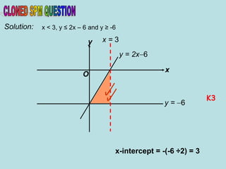
112. y
x
O
y = 2x6
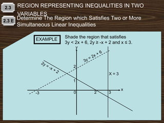
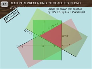
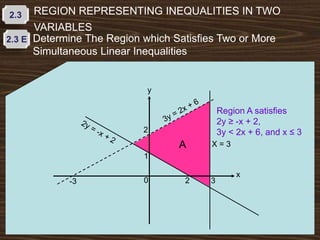
On the graphs provided, shade the region which satisfies
the three inequalities x < 3, y ≤ 2x – 6 and y ≥ -6
[3 marks]
y = 6

113. y
x
O
y = 2x6
y = 6
Solution:
x = 3
K3
x-intercept = -(-6 ÷2) = 3
x < 3, y ≤ 2x – 6 and y ≥ -6

114. On the graphs provided, shade the region which satisfies
the three inequalities y ≤ x - 4, y ≤ -3x + 12 and y > -4
[3 marks]
y
x
y = 3x+12
O
y = x4

115. y
x
y = 3x+12
O
y = x4
y = 4
Solution:
K3
y-intercept =-4
y ≤ x - 4, y ≤ -3x + 12 and y > -4

116. SPM 2003 PAPER 2
REFER TO QUESTION
NO. 12

117. 12. ( a )
x -4 -2.5 -1 -0.5 0.5 1 2 3.2 4
y 1 1.6 8 -8 -4 -1.25 -1
4
2
  K1K1
y = -4
( )
=
y = -4
( )
=
-1
4 -2-2

118. 1 2 3 4-1-2-3-4 0
y
x
2
4
6
8
-2
-4
-6
-8
X
X
X
X
X
X
X
X
X

K1
 


K1N1


 
K1N1

12(b)

119. 12. ( a )
x -4 -2.5 -1 -0.5 0.5 1 2 3.2 4
y 1 1.6 8 -8 -4 -1.25 -14 2
 K1K0

120. 1 2 3 4-1-2-3-4 0
y
x
2
4
6
8
-2
-4
-6
-8
X
X
X
X
X
X
X
X
X

K1
 


K1N1



K1 N0

12(b)

121. x
y
0 1 2 3 4
8
6
4
2
-2
-4
-6
-8
-4 -3 -2 -1
x
x
x
x
x
x
x
12. ( c )
x
-2.2
-1.2
1.8
3.4
( i ) y = -2.2
( ii ) x = -1.2
 P1
 P1

122. 12. (d)
x
y
0 1 2 3 4
8
6
4
2
-2
-4
-6
-8
-4 -3 -2 -1
x
x
x
x
x
x
x
x
y = -2x - 3
-2.4
0.8
 K1K1
x = - 2.4
x = 0.8

 N1
4 = 2x + 3
x
- 4 = -2x - 3
x