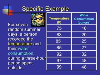
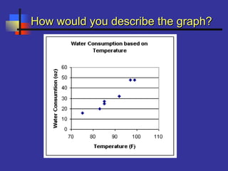
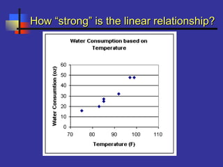
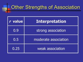
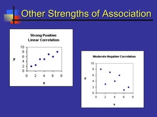
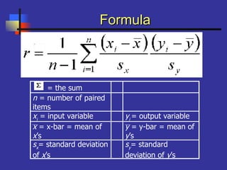
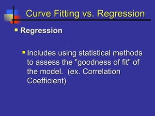
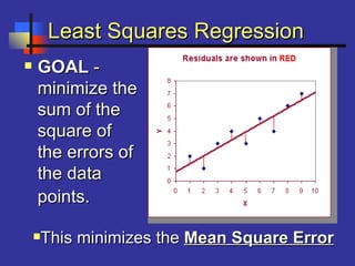
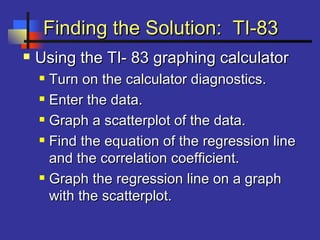
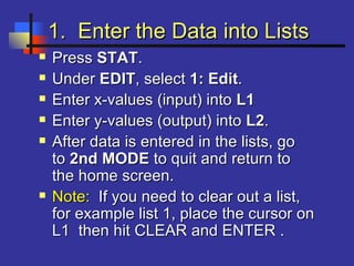
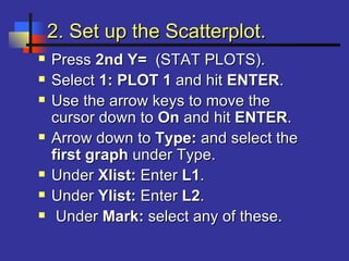
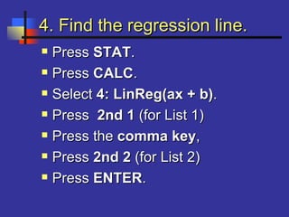
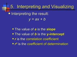
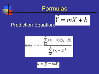
This document introduces correlation and regression. It defines correlation as a measure of the association between two numerical variables and discusses how the Pearson correlation coefficient measures both the direction and strength of the linear relationship between two variables. Regression is introduced as a statistical method for finding the line of best fit for one variable based on another. Simple linear regression finds the line of best fit for one dependent variable based on one independent variable. The document provides steps for performing simple linear regression using a TI-83 graphing calculator.

1. Introduction toIntroduction to
Correlation and RegressionCorrelation and Regression
Ginger Holmes Rowell, Ph. D.Ginger Holmes Rowell, Ph. D.
Associate Professor of MathematicsAssociate Professor of Mathematics
Middle Tennessee State UniversityMiddle Tennessee State University

2. OutlineOutline
 IntroductionIntroduction
 Linear CorrelationLinear Correlation
 RegressionRegression
 Simple LinearSimple Linear
RegressionRegression
 Using the TI-83Using the TI-83
 Model/FormulasModel/Formulas

3. Outline continuedOutline continued
 ApplicationsApplications
 Real-life ApplicationsReal-life Applications
 Practice ProblemsPractice Problems
 Internet ResourcesInternet Resources
 AppletsApplets
 Data SourcesData Sources

4. CorrelationCorrelation
 CorrelationCorrelation
 A measure of association betweenA measure of association between
two numerical variables.two numerical variables.
 Example (positive correlation)Example (positive correlation)
 Typically, in the summer as theTypically, in the summer as the
temperature increases people aretemperature increases people are
thirstier.thirstier.

5. Specific ExampleSpecific Example
For sevenFor seven
random summerrandom summer
days, a persondays, a person
recorded therecorded the
temperaturetemperature andand
theirtheir waterwater
consumptionconsumption,,
during a three-hourduring a three-hour
period spentperiod spent
outside.outside.
Temperature
(F)
Water
Consumption
(ounces)
75 16
83 20
85 25
85 27
92 32
97 48
99 48

6. How would you describe the graph?How would you describe the graph?

7. How “strong” is the linear relationship?How “strong” is the linear relationship?

8. Measuring the RelationshipMeasuring the Relationship
Pearson’s SamplePearson’s Sample
Correlation Coefficient,Correlation Coefficient, rr
measures themeasures the directiondirection and theand the
strengthstrength of the linear associationof the linear association
between two numerical pairedbetween two numerical paired
variables.variables.

9. Direction of AssociationDirection of Association
Positive CorrelationPositive Correlation NegativeNegative
CorrelationCorrelation

10. Strength of Linear AssociationStrength of Linear Association
r
value
Interpretation
1
perfect positive linear
relationship
0 no linear relationship
-1
perfect negative linear
relationship

11. Strength of Linear AssociationStrength of Linear Association

12. Other Strengths of AssociationOther Strengths of Association
r value Interpretation
0.9 strong association
0.5 moderate association
0.25 weak association

13. Other Strengths of AssociationOther Strengths of Association

14. FormulaFormula
= the sum
n = number of paired
items
xi
= input variable yi
= output variable
x = x-bar = mean of
x’s
y = y-bar = mean of
y’s
sx
= standard deviation
of x’s
sy
= standard
deviation of y’s
sum

15. RegressionRegression
 RegressionRegression
 Specific statistical methodsSpecific statistical methods forfor
finding the “line of best fit” for onefinding the “line of best fit” for one
response (dependent) numericalresponse (dependent) numerical
variable based on one or morevariable based on one or more
explanatory (independent)explanatory (independent)
variables.variables.

16. Curve Fitting vs. RegressionCurve Fitting vs. Regression
 RegressionRegression
 Includes using statistical methodsIncludes using statistical methods
to assess the "goodness of fit" ofto assess the "goodness of fit" of
the model. (ex. Correlationthe model. (ex. Correlation
Coefficient)Coefficient)

17. Regression: 3 Main PurposesRegression: 3 Main Purposes
 To describeTo describe (or model)(or model)
 To predictTo predict ((or estimate)or estimate)
 To controlTo control (or administer)(or administer)

18. Simple Linear RegressionSimple Linear Regression
 Statistical method for findingStatistical method for finding
 the “line of best fit”the “line of best fit”
 for one response (dependent)for one response (dependent)
numerical variablenumerical variable
 based on one explanatorybased on one explanatory
(independent) variable.(independent) variable.

19. Least Squares RegressionLeast Squares Regression
 GOALGOAL --
minimize theminimize the
sum of thesum of the
square ofsquare of
the errors ofthe errors of
the datathe data
points.points.
This minimizes theThis minimizes the Mean Square ErrorMean Square Error

20. ExampleExample
 Plan an outdoor party.Plan an outdoor party.
 EstimateEstimate number of soft drinks tonumber of soft drinks to
buy per person, based on how hotbuy per person, based on how hot
the weather is.the weather is.
 Use Temperature/Water data andUse Temperature/Water data and
regressionregression..

21. Steps to Reaching a SolutionSteps to Reaching a Solution
 Draw a scatterplot of the data.Draw a scatterplot of the data.

22. Steps to Reaching a SolutionSteps to Reaching a Solution
 Draw a scatterplot of the data.Draw a scatterplot of the data.
 Visually, consider the strength of theVisually, consider the strength of the
linear relationship.linear relationship.

23. Steps to Reaching a SolutionSteps to Reaching a Solution
 Draw a scatterplot of the data.Draw a scatterplot of the data.
 Visually, consider the strength of theVisually, consider the strength of the
linear relationship.linear relationship.
 If the relationship appears relativelyIf the relationship appears relatively
strong, find the correlation coefficientstrong, find the correlation coefficient
as a numerical verification.as a numerical verification.

24. Steps to Reaching a SolutionSteps to Reaching a Solution
 Draw a scatterplot of the data.Draw a scatterplot of the data.
 Visually, consider the strength of theVisually, consider the strength of the
linear relationship.linear relationship.
 If the relationship appears relativelyIf the relationship appears relatively
strong, find the correlation coefficientstrong, find the correlation coefficient
as a numerical verification.as a numerical verification.
 If the correlation is still relativelyIf the correlation is still relatively
strong, then find the simple linearstrong, then find the simple linear
regression line.regression line.

25. Our Next StepsOur Next Steps
 Learn to Use the TI-83 forLearn to Use the TI-83 for
Correlation and Regression.Correlation and Regression.
 Interpret the Results (in theInterpret the Results (in the
Context of the Problem).Context of the Problem).

26. Finding the Solution: TI-83Finding the Solution: TI-83
 Using the TI- 83 graphing calculatorUsing the TI- 83 graphing calculator
 Turn on the calculator diagnostics.Turn on the calculator diagnostics.
 Enter the data.Enter the data.
 Graph a scatterplot of the data.Graph a scatterplot of the data.
 Find the equation of the regression lineFind the equation of the regression line
and the correlation coefficient.and the correlation coefficient.
 Graph the regression line on a graphGraph the regression line on a graph
with the scatterplot.with the scatterplot.

27. Preliminary StepPreliminary Step
 Turn the Diagnostics On.Turn the Diagnostics On.
 PressPress 2nd 02nd 0 (for Catalog).(for Catalog).
 Scroll down toScroll down to DiagnosticOnDiagnosticOn. The. The
marker points to the right of themarker points to the right of the
words.words.
 PressPress ENTERENTER. Press. Press ENTERENTER
again.again.
 The wordThe word DoneDone should appear onshould appear on
the right hand side of the screen.the right hand side of the screen.

28. ExampleExample
Temperature
(F)
Water
Consumption
(ounces)
75 16
83 20
85 25
85 27
92 32
97 48
99 48

29. 1. Enter the Data into Lists1. Enter the Data into Lists
 PressPress STATSTAT..
 UnderUnder EDITEDIT, select, select 1: Edit1: Edit..
 Enter x-values (input) intoEnter x-values (input) into L1L1
 Enter y-values (output) intoEnter y-values (output) into L2L2..
 After data is entered in the lists, goAfter data is entered in the lists, go
toto 2nd MODE2nd MODE to quit and return toto quit and return to
the home screen.the home screen.
 Note:Note: If you need to clear out a list,If you need to clear out a list,
for example list 1, place the cursor onfor example list 1, place the cursor on
L1 then hit CLEAR and ENTER .L1 then hit CLEAR and ENTER .

30. 2. Set up the Scatterplot.2. Set up the Scatterplot.
 PressPress 2nd Y=2nd Y= (STAT PLOTS).(STAT PLOTS).
 SelectSelect 1: PLOT 11: PLOT 1 and hitand hit ENTERENTER..
 Use the arrow keys to move theUse the arrow keys to move the
cursor down tocursor down to OnOn and hitand hit ENTERENTER..
 Arrow down toArrow down to Type:Type: and select theand select the
first graphfirst graph under Type.under Type.
 UnderUnder Xlist:Xlist: EnterEnter L1L1..
 UnderUnder Ylist:Ylist: EnterEnter L2L2..
 UnderUnder Mark:Mark: select any of these.select any of these.

31. 3. View the Scatterplot3. View the Scatterplot
 PressPress 2nd MODE2nd MODE to quit andto quit and
return to the home screen.return to the home screen.
 To plot the points, pressTo plot the points, press ZOOMZOOM
and selectand select 9: ZoomStat9: ZoomStat..
 The scatterplot will then beThe scatterplot will then be
graphed.graphed.

32. 4. Find the regression line.4. Find the regression line.
 PressPress STATSTAT..
 PressPress CALCCALC..
 SelectSelect 4: LinReg(ax + b)4: LinReg(ax + b)..
 PressPress 2nd 12nd 1 (for List 1)(for List 1)
 Press thePress the comma keycomma key,,
 PressPress 2nd 22nd 2 (for List 2)(for List 2)
 PressPress ENTERENTER..

33. 5. Interpreting and Visualizing5. Interpreting and Visualizing
 Interpreting the result:Interpreting the result:
y = ax + by = ax + b
 The valueThe value ofof aa is theis the slopeslope
 The value ofThe value of bb is theis the y-intercepty-intercept
 rr is theis the correlation coefficientcorrelation coefficient
 rr22
is theis the coefficient of determinationcoefficient of determination

34. 5. Interpreting and Visualizing5. Interpreting and Visualizing
 Write down the equation of theWrite down the equation of the
line in slope intercept form.line in slope intercept form.
 PressPress Y=Y= and enter the equationand enter the equation
under Y1. (Clear all otherunder Y1. (Clear all other
equations.)equations.)
 PressPress GRAPHGRAPH and the line willand the line will
be graphed through the databe graphed through the data
points.points.

35. Questions ???Questions ???

36. Interpretation in ContextInterpretation in Context
 Regression Equation:Regression Equation:
y=1.5*x - 96.9y=1.5*x - 96.9
Water Consumption =Water Consumption =
1.5*Temperature - 96.91.5*Temperature - 96.9

37. Interpretation in ContextInterpretation in Context
 Slope = 1.5 (ounces)/(degrees F)Slope = 1.5 (ounces)/(degrees F)
 for each 1 degree F increase infor each 1 degree F increase in
temperature, you expect an increasetemperature, you expect an increase
of 1.5 ounces of water drank.of 1.5 ounces of water drank.

38. Interpretation in ContextInterpretation in Context
y-intercept = -96.9y-intercept = -96.9
 For this example,For this example,
when the temperature is 0 degrees F,when the temperature is 0 degrees F,
then a person would drink about -97then a person would drink about -97
ounces of water.ounces of water.
 That does not make any sense!That does not make any sense!
 Our model is not applicable for x=0.Our model is not applicable for x=0.

39. Prediction ExamplePrediction Example
 PredictPredict the amount ofthe amount of
water a person would drink when thewater a person would drink when the
temperature istemperature is 95 degrees F.95 degrees F.
 Solution:Solution: Substitute the value of x=95Substitute the value of x=95
(degrees F) into the regression equation(degrees F) into the regression equation
and solve for y (water consumption).and solve for y (water consumption).
If x=95, y=1.5*95 - 96.9 =If x=95, y=1.5*95 - 96.9 = 45.6 ounces.45.6 ounces.

40. Strength of the Association:Strength of the Association: rr22
 Coefficient of Determination –Coefficient of Determination – rr22
 General Interpretation:General Interpretation: TheThe
coefficient of determination tells thecoefficient of determination tells the
percent of the variationpercent of the variation in thein the
response variable that isresponse variable that is explainedexplained
(determined) by the model and the(determined) by the model and the
explanatory variable.explanatory variable.

41. Interpretation ofInterpretation of rr22
 Example:Example: rr22
=92.7%.=92.7%.
 Interpretation:Interpretation:
 Almost 93% of the variability in theAlmost 93% of the variability in the
amount of water consumed isamount of water consumed is
explained by outside temperatureexplained by outside temperature
using this model.using this model.
 Note: Therefore 7% of theNote: Therefore 7% of the
variation in the amount of watervariation in the amount of water
consumed is not explained by thisconsumed is not explained by this
model using temperature.model using temperature.

42. Questions ???Questions ???

43. Simple Linear Regression ModelSimple Linear Regression Model
The model forThe model for
simple linear regression issimple linear regression is
There are mathematical assumptions behindThere are mathematical assumptions behind
the concepts thatthe concepts that
we are covering today.we are covering today.

44. FormulasFormulas
Prediction Equation:Prediction Equation:

45. Real Life ApplicationsReal Life Applications
Cost Estimating for Future SpaceCost Estimating for Future Space
Flight Vehicles (MultipleFlight Vehicles (Multiple
Regression)Regression)

46. Nonlinear ApplicationNonlinear Application
Predicting when Solar Maximum WillPredicting when Solar Maximum Will
OccurOccur
http://science.msfc.nasa.gov/ssl/pad/http://science.msfc.nasa.gov/ssl/pad/
solar/predict.htmsolar/predict.htm

47. Real Life ApplicationsReal Life Applications
 Estimating Seasonal Sales forEstimating Seasonal Sales for
Department Stores (Periodic)Department Stores (Periodic)

48. Real Life ApplicationsReal Life Applications
 Predicting Student Grades BasedPredicting Student Grades Based
on Time Spent Studyingon Time Spent Studying

49. Real Life ApplicationsReal Life Applications
 . . .. . .
 What ideas can you think of?What ideas can you think of?
 What ideas can you think of thatWhat ideas can you think of that
your students will relate to?your students will relate to?

50. Practice ProblemsPractice Problems
 Measure Height vs. Arm SpanMeasure Height vs. Arm Span
 Find line of best fit for height.Find line of best fit for height.
 Predict height forPredict height for
one student not inone student not in
data set. Checkdata set. Check
predictability of model.predictability of model.

51. Practice ProblemsPractice Problems
 Is there any correlation betweenIs there any correlation between
shoe size and height?shoe size and height?
 Does gender make a differenceDoes gender make a difference
in this analysis?in this analysis?

52. Practice ProblemsPractice Problems
 Can the number of pointsCan the number of points
scored in a basketball game bescored in a basketball game be
predicted bypredicted by
 The time a player plays inThe time a player plays in
the game?the game?
 By the player’s height?By the player’s height?
Idea modified from Steven King, Aiken,Idea modified from Steven King, Aiken,
SC. NCTM presentation 1997.)SC. NCTM presentation 1997.)

53. ResourcesResources
 Data Analysis and StatisticsData Analysis and Statistics..
Curriculum and EvaluationCurriculum and Evaluation
Standards for School Mathematics.Standards for School Mathematics.
Addenda Series, Grades 9-12.Addenda Series, Grades 9-12.
NCTM. 1992.NCTM. 1992.
 Data and Story LibraryData and Story Library. Internet. Internet
Website.Website.
http://lib.stat.cmu.edu/DASL/http://lib.stat.cmu.edu/DASL/
2001.2001.

54. Internet ResourcesInternet Resources
 CorrelationCorrelation
 Guessing CorrelationsGuessing Correlations - An- An
interactive site that allows you tointeractive site that allows you to
try to match correlation coefficientstry to match correlation coefficients
to scatterplots. University of Illinois,to scatterplots. University of Illinois,
Urbanna Champaign StatisticsUrbanna Champaign Statistics
Program.Program.
http://www.stat.uiuc.edu/~stat100/java/guhttp://www.stat.uiuc.edu/~stat100/java/gu

55. Internet ResourcesInternet Resources
 RegressionRegression
 Effects of adding anEffects of adding an
OutlierOutlier..
W. West, University of SouthW. West, University of South
Carolina.Carolina.
http://www.stat.sc.edu/~west/javahtml/Rhttp://www.stat.sc.edu/~west/javahtml/R

56. Internet ResourcesInternet Resources
 RegressionRegression
 Estimate the Regression LineEstimate the Regression Line..
Compare the mean square errorCompare the mean square error
from different regression lines. Canfrom different regression lines. Can
you find the minimum mean squareyou find the minimum mean square
error? Rice University Virtualerror? Rice University Virtual
Statistics Lab.Statistics Lab.
http://www.ruf.rice.edu/~lane/stat_sim/reghttp://www.ruf.rice.edu/~lane/stat_sim/reg

57. Internet Resources: Data SetsInternet Resources: Data Sets
 Data and Story Library.Data and Story Library.
Excellent source for small data sets.Excellent source for small data sets.
Search for specific statistical methodsSearch for specific statistical methods
(e.g. boxplots, regression) or for data(e.g. boxplots, regression) or for data
concerning a specific field of interestconcerning a specific field of interest
(e.g. health, environment, sports).(e.g. health, environment, sports).
http://lib.stat.cmu.edu/DASL/http://lib.stat.cmu.edu/DASL/

58. Internet Resources: Data SetsInternet Resources: Data Sets
 FEDSTATS.FEDSTATS. "The gateway to"The gateway to
statistics from over 100 U.S. Federalstatistics from over 100 U.S. Federal
agencies"agencies" http://www.fedstats.gov/http://www.fedstats.gov/
 "Kid's Pages.""Kid's Pages." (not all related to(not all related to
statistics)statistics)
http://www.fedstats.gov/kids.htmlhttp://www.fedstats.gov/kids.html

59. Internet ResourcesInternet Resources
 OtherOther
 Statistics Applets. Using WebStatistics Applets. Using Web
Applets to Assist in StatisticsApplets to Assist in Statistics
Instruction. Robin Lock, St.Instruction. Robin Lock, St.
Lawrence University.Lawrence University.
http://it.stlawu.edu/~rlock/maa99/http://it.stlawu.edu/~rlock/maa99/

60. Internet ResourcesInternet Resources
 OtherOther
 Ten Websites Every StatisticsTen Websites Every Statistics
Instructor Should Bookmark.Instructor Should Bookmark.
Robin Lock, St. LawrenceRobin Lock, St. Lawrence
University.University.
http://it.stlawu.edu/~rlock/10sites.htmhttp://it.stlawu.edu/~rlock/10sites.htm

61. For More Information…For More Information…
On-line version of this presentationOn-line version of this presentation
http://www.mtsu.edu/~statshttp://www.mtsu.edu/~stats
/corregpres/index.html/corregpres/index.html
More information about regressionMore information about regression
VisitVisit STATS @ MTSUSTATS @ MTSU web siteweb site
http://www.mtsu.edu/~statshttp://www.mtsu.edu/~stats