Download as PDF, PPTX

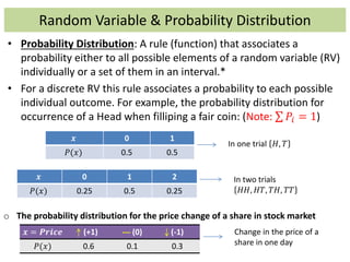
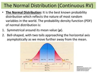
![Probability Distributions (Continuous)
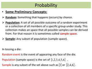
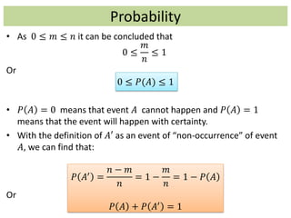
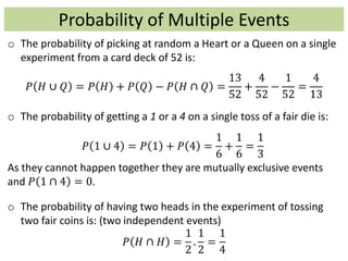
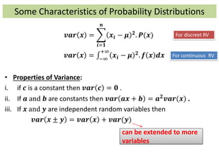
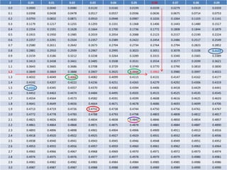
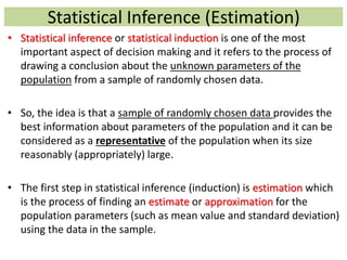
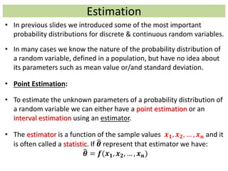
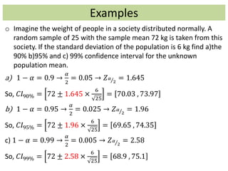
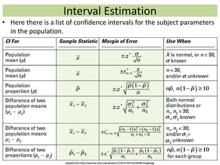
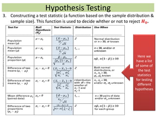
• The probability that a continuous random variable chooses
just one of its values in its domain is zero, because the number
of all possible outcomes 𝒏 is infinite and
𝒎
∞
→ 𝟎.
• For the above reason, the probability of a continuous random
variable need to be calculated in an interval.
• The probability distribution of a continuous random variable is
often called a probability density function (PDF) or simply
probability function and it is usually shown by 𝒇(𝒙) and it has
following properties:
I. 𝑓(𝑥) ≥ 0 (similar to 𝑷(𝒙) ≥ 𝟎 for discrete RV*)
II. −∞
+∞
𝑓 𝑥 𝑑𝑥 = 1 (similar to 𝑷 𝒙 = 𝟏 for discrete RV)
III. 𝑎
𝑏
𝑓 𝑥 𝑑𝑥 = 𝑃 𝑎 ≤ 𝑥 ≤ 𝑏 = 𝐹 𝑏 − 𝐹 𝑎 (probability
given to set of values in an interval [a,b] )**](https://image.slidesharecdn.com/statisticsrecap-150114144147-conversion-gate01/85/Statistics-recap-14-320.jpg)
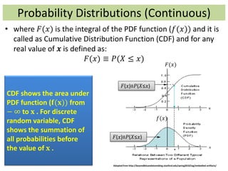
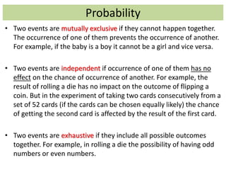
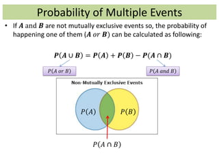
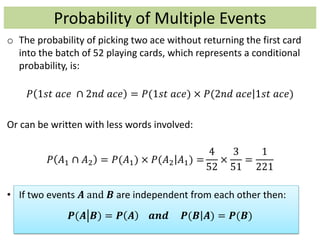
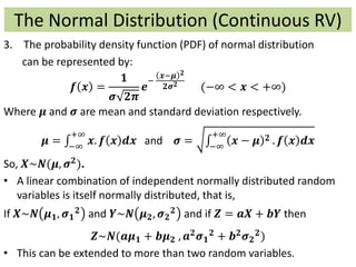
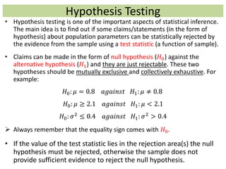
![Some Characteristics of Probability Distributions
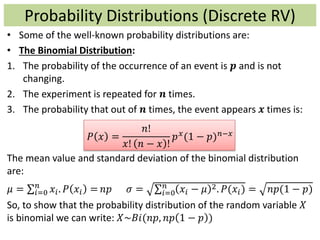
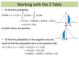
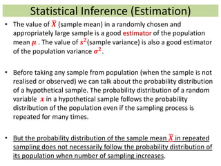
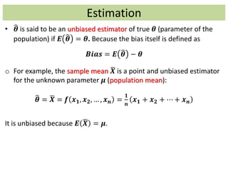
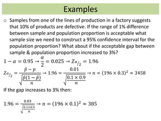
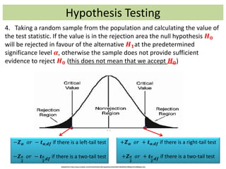
v. If 𝒈 𝒙 is a function of random variable 𝒙 then
𝑬 𝒈 𝒙 = 𝒈 𝒙 . 𝑷(𝒙)
𝑬 𝒈 𝒙 = 𝒈 𝒙 . 𝒇 𝒙 𝒅𝒙
• Variance: To measure how random variable 𝒙 is dispersed around
its expected value, variance can help. If we show 𝑬 𝒙 = 𝝁 , then
𝒗𝒂𝒓 𝒙 = 𝝈 𝟐 = 𝑬[ 𝒙 − 𝑬 𝒙
𝟐
]
= 𝑬[ 𝒙 − 𝝁 𝟐]
= 𝑬[𝒙 𝟐 − 𝟐𝒙𝝁 + 𝝁 𝟐]
= 𝑬 𝒙 𝟐 − 𝟐𝝁𝑬 𝒙 + 𝝁 𝟐
= 𝑬 𝒙 𝟐 − 𝝁 𝟐
For discreet RV
For continuous RV](https://image.slidesharecdn.com/statisticsrecap-150114144147-conversion-gate01/85/Statistics-recap-18-320.jpg)
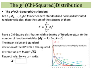
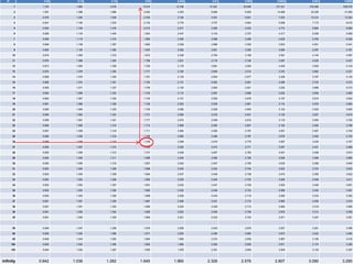
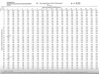

1) The document provides an overview of key concepts in probability and statistics, including random variables, probability distributions, and characteristics of distributions such as expected value and variance. 2) It defines key probability terms such as population, sample, mutually exclusive events, independent events, and exhaustive events. It also covers how to calculate the probability of single and multiple events. 3) The document distinguishes between discrete and continuous random variables and probability distributions. It explains how probability distributions associate probabilities with individual outcomes for discrete variables but use probability density functions to provide probabilities over intervals for continuous variables.


