pid controller

1. Review
of
Feedback Control System

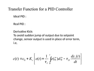
2. Transfer Function for a PID Controller
Ideal PID :
Real PID :
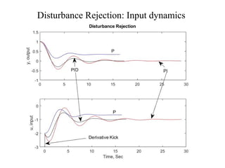
Derivative Kick:
To avoid sudden jump of output due to setpoint
change, sensor output is used in place of error term,
i.e,
0
0
( )
1
( ) ( ) ( )
t
s
c D
I
dy t
c t c K e t e d
dt
  

 
   
 
 


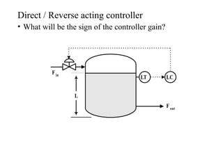
3. Direct / Reverse acting controller
• What will be the sign of the controller gain?
Fout
Fin
L
LC
LT

4. Guidelines for Selecting Direct and Reverse
Acting PID’s
• Consider a direct acting final control element to be
positive and reverse to be negative.
• If the sign of the product of the final control
element and the process gain is positive, use the
reverse acting PID algorithm.
• If the sign of the product is negative, use the direct
acting PID algorithm
• If control signal goes to a control valve with a valve
positioner, the actuator is considered direct acting.

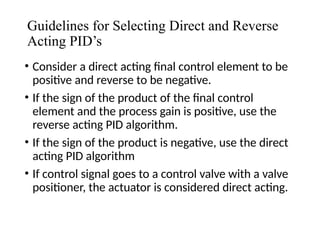
5. Level Control Example
• Process gain is positive
because when flow in is
increased, the level
increases.
• If the final control
element is direct acting,
use reverse acting PID.
• For reverse acting final
control element, use
direct acting PID.
Fout
Fin
L
LC
LT

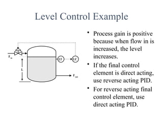
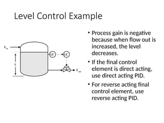
6. Level Control Example
Fout
Fin
L
LC
LT
• Process gain is negative
because when flow out is
increased, the level
decreases.
• If the final control
element is direct acting,
use direct acting PID.
• For reverse acting final
control element, use
reverse acting PID.

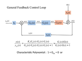
7. General Feedback Control Loop
GP(s)
Ga(s)
GC(s)
KS
GS(s)
Gd(s)
d(s)
ysp(s)
+
-
+
+
u(s) y(s)
c(s)
e(s)
yS(s)
1
)
(
)
(
)
(
)
(
1
)
(
)
(
)
(
)
(
)
(
)
(
)
(
)
(
)
(




s
G
s
G
s
G
s
G
s
G
s
G
s
G
s
G
s
G
s
G
s
G
K
s
y
s
y
c
c
s
c
a
p
c
a
p
S
sp
Characteristic Polynomial : 1 + GOL = 0 or

8. Controller actions on feedback dynamics
Process G(s) : Controller : Proportional, ;
Matlab:
s=tf(‘s’); g=1/(s+1)^3;
step(g); hold on
for kc=[0.5:0.5:2],
gcl=feedback(kc*g,1);
step(gcl);
end

9. Proportional Control
Important points:
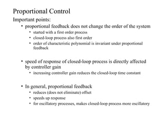
• proportional feedback does not change the order of the system
• started with a first order process
• closed-loop process also first order
• order of characteristic polynomial is invariant under proportional
feedback
• speed of response of closed-loop process is directly affected
by controller gain
• increasing controller gain reduces the closed-loop time constant
• In general, proportional feedback
• reduces (does not eliminate) offset
• speeds up response
• for oscillatory processes, makes closed-loop process more oscillatory

10. Controller actions on feedback dynamics
Process G(s) : Controller : PI (I varying) ;
Matlab:
figure; hold on; kc=2;
for Ti=[2:1:5],
gc=tf(kc*[1,1/Ti],[1,0]);
gcl=feedback(gc*g,1);
step(gcl);
end

11. Proporional - Integral Control
Important points:
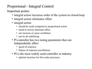
• integral action increases order of the system in closed-loop
• integral action eliminates offset
• integral action
• should be small compared to proportional action
• tuned to slowly eliminate offset
• can increase or cause oscillation
• can be de-stabilizing
• PI controller has two tuning parameters that can
independently affect
• speed of response
• Nature of response (oscillation)
• PI is the most widely used controller in industry
• optimal structure for first order processes

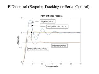
12. Controller actions on feedback dynamics
Process G(s) : Controller : PD, ;
Matlab:
figure; hold on; kc=2;
for Td=[0:0.2:0.8],
gc=tf(kc*[Td,1],[1]);
gcl=feedback(gc*g,1);
step(gcl); end

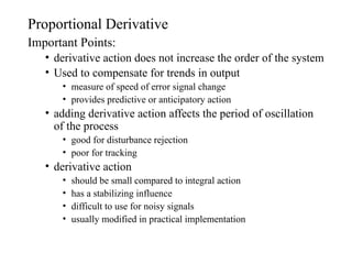
13. Proportional Derivative
Important Points:
• derivative action does not increase the order of the system
• Used to compensate for trends in output
• measure of speed of error signal change
• provides predictive or anticipatory action
• adding derivative action affects the period of oscillation
of the process
• good for disturbance rejection
• poor for tracking
• derivative action
• should be small compared to integral action
• has a stabilizing influence
• difficult to use for noisy signals
• usually modified in practical implementation

14. PID control (Setpoint Tracking or Servo Control)

15. Disturbance Rejection: Input dynamics

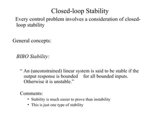
16. Closed-loop Stability
Every control problem involves a consideration of closed-
loop stability
General concepts:
BIBO Stability:
“ An (unconstrained) linear system is said to be stable if the
output response is bounded for all bounded inputs.
Otherwise it is unstable.”
Comments:
• Stability is much easier to prove than instability
• This is just one type of stability

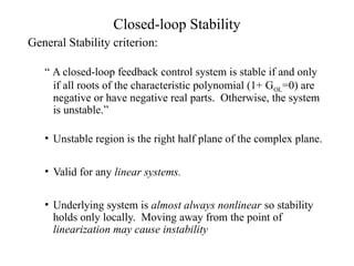
17. Closed-loop Stability
General Stability criterion:
“ A closed-loop feedback control system is stable if and only
if all roots of the characteristic polynomial (1+ GOL=0) are
negative or have negative real parts. Otherwise, the system
is unstable.”
• Unstable region is the right half plane of the complex plane.
• Valid for any linear systems.
• Underlying system is almost always nonlinear so stability
holds only locally. Moving away from the point of
linearization may cause instability

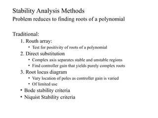
18. Stability Analysis Methods
Problem reduces to finding roots of a polynomial
Traditional:
1. Routh array:
• Test for positivity of roots of a polynomial
2. Direct substitution
• Complex axis separates stable and unstable regions
• Find controller gain that yields purely complex roots
3. Root locus diagram
• Vary location of poles as controller gain is varied
• Of limited use
• Bode stability criteria
• Niquist Stability criteria

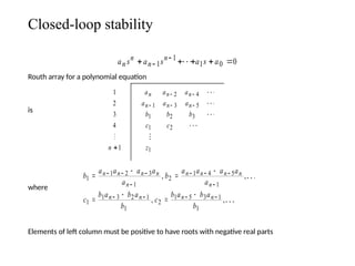
19. Closed-loop stability
Routh array for a polynomial equation
is
where
Elements of left column must be positive to have roots with negative real parts
a s a s a s a
n
n
n
n
    


1
1
1 0 0

a a a
a a a
b b b
c c
z
n n n
n n n
 
  
2 4
1 3 5
1 2 3
1 2
1





1
2
3
4
1

n 
b
a a a a
a
b
a a a a
a
c
b a b a
b
c
b a b a
b
n n n n
n
n n n n
n
n n n n
1
1 2 3
1
2
1 4 5
1
1
1 3 2 1
1
2
1 5 3 1
1








  

  

   
, ,
, ,



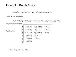
20. Example: Routh Array
Characteristic polynomial
Polynomial Coefficients
Routh Array
• Closed-loop system is unstable
2 36 1 49 0 58 1 21 0 42 0 78 0
5 4 3 2
. . . . . .
s s s s s
     
a a a
a a a
b b b
c c
d d
e
5 3 1
4 2 0
1 2 3
1 2
1 2
1
2 36 0 58 0 42
1 49 1 21 0 78
2 50 0 82 0
0 72 0 78
1 89 0
0 78
( . ) ( . ) ( . )
( . ) ( . ) ( . )
( . ) ( . ) ( )
( . ) ( . )
( . ) ( )
( . )

 
a a a a a a
5 4 3 2 1 0
2 36 1 49 0 58 1 21 0 42 0 78
      
. , . , . , . , . , .
1
2
3
4
5
6

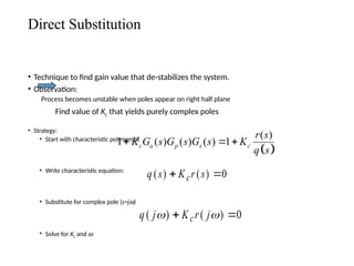
21. Direct Substitution
• Technique to find gain value that de-stabilizes the system.
• Observation:
Process becomes unstable when poles appear on right half plane
Find value of Kc that yields purely complex poles
• Strategy:
• Start with characteristic polynomial
• Write characteristic equation:
• Substitute for complex pole (s=jw)
• Solve for Kc and w
q j K r j
c
( ) ( )
 
 0
 
( )
1 ( ) ( ) ( ) 1
c a p s c
r s
K G s G s G s K
q s
  
q s K r s
c
( ) ( )
 0

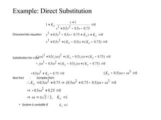
22. Example: Direct Substitution
Characteristic equation
Substitution for s=jw
Real Part : Complex Part:
• System is unstable if
1
1
0 5 0 5 0 75
0
0 5 0 5 0 75 0
0 5 0 5 0 75 0
3 2
3 2
3 2


  

     
     
K
s
s s s
s s s K s K
s s K s K
c
c c
c c
. . .
. . .
. ( . ) ( . )
( ) . ( ) ( . ) ( . )
. ( . ) ( . )
j j K j K
j K j K
c c
c c
  
  
3 2
3 2
0 5 0 5 0 75 0
0 5 0 5 0 75 0
     
      
   
0 5 0 75 0
2
. .
 Kc ( . )
Kc   
0 5 0
3
 
       
   
  
K
K
c
c
0 5 0 75 0 5 0 75 0 5 0
0 5 0 25 0
2 2 1
2 2 3
2
. . ( . . . )
. .
/ ,
   


Kc 1

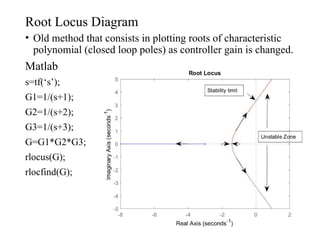
23. Root Locus Diagram
• Old method that consists in plotting roots of characteristic
polynomial (closed loop poles) as controller gain is changed.
Matlab
s=tf(‘s’);
G1=1/(s+1);
G2=1/(s+2);
G3=1/(s+3);
G=G1*G2*G3;
rlocus(G);
rlocfind(G);

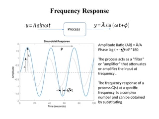
24. Frequency Response
Process
𝑢=𝐴𝑠𝑖𝑛𝜔𝑡 𝑦=^
𝐴 sin⁡(𝜔𝑡+𝜙)
0 20 40 60 80 100
-2
-1.5
-1
-0.5
0
0.5
1
1.5
2
Sinusoidal Response
Time (seconds)
Amplitude
A
Â
t
Amplitude Ratio (AR) = Â/A
Phase lag ( = -t/P*180
The process acts as a “filter”
or “amplifier” that attenuates
or amplifies the input at
frequency .
The frequency response of a
process G(s) at a specific
frequency is a complex
number and can be obtained
by substituting
P

25. Frequency Response
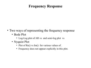
• Two ways of representing the frequency response
• Bode Plot
• Log-Log plot of AR vs and semi-log plot vs
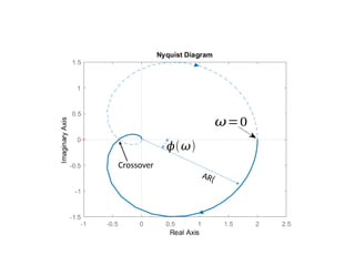
• Nyquist Plot
• Plot of Re() vs Im() for various values of .
• Frequency does not appear explicitly in this plot.

26. Bode Plot
10
-5
10
0
Magnitude
(abs)
10
-2
10
-1
10
0
10
1
10
2
-360
-315
-270
-225
-180
-135
-90
-45
0
Phase
(deg)
Bode Diagram
Frequency (rad/s)
Crossover
Frequency
Corner Frequency
Meeting pt of LFA and HFA
Steady state gain:
Bandwidth, , defines
the highest
frequency at which
the process displays
no attenuation. It is
calculated based on
the frequency when
amplitude reaches
0.707 K.
Roll-off is slope of
decaying AR at high
frequencies.

27. 𝜔=0
Crossover
AR(
𝜙(𝜔)

28. Bode Stability Criterion
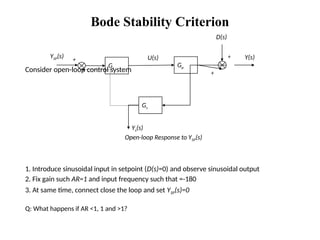
Consider open-loop control system
1. Introduce sinusoidal input in setpoint (D(s)=0) and observe sinusoidal output
2. Fix gain such AR=1 and input frequency such that =-180
3. At same time, connect close the loop and set YSP(s)=0
Q: What happens if AR <1, 1 and >1?
Open-loop Response to YSP(s)
Gp
Gc
Gs
D(s)
Y(s)
Ys(s)
YSP(s) U(s)
+
-
+
+

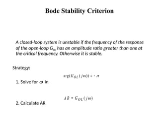
29. Bode Stability Criterion
A closed-loop system is unstable if the frequency of the response
of the open-loop GOL has an amplitude ratio greater than one at
the critical frequency. Otherwise it is stable.
Strategy:
1. Solve for w in
2. Calculate AR
arg( ( ))
G j
OL  
 
AR G j
OL
 ( )


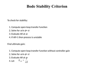
30. Bode Stability Criterion
To check for stability:
1. Compute open-loop transfer function
2. Solve for w in f=-p
3. Evaluate AR at w
4. If AR>1 then process is unstable
Find ultimate gain:
1. Compute open-loop transfer function without controller gain
2. Solve for w in f=-p
3. Evaluate AR at w
4. Let K
AR
cu 
1

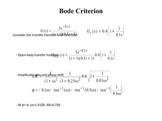
31. Bode Criterion
Consider the transfer function and controller
- Open-loop transfer function
- Amplitude ratio and phase shift
- At f=-p, w=1.4128, AR=6.746
G s
e
s s
s
( )
( )( . )
.

 

5
1 0 5 1
0 1
G s
s
c ( ) .
.
 






0 4 1
1
0 1
G s
e
s s s
OL
s
( )
( )( . )
.
.
.

 








5
1 0 5 1
0 4 1
1
0 1
0 1
AR 
 

     





  
5
1
1
1 0 25
0 4 1
1
0 01
0 1 0 5
1
0 1
2 2 2
1 1 1
  
   

.
.
.
. tan ( ) tan ( . ) tan
.

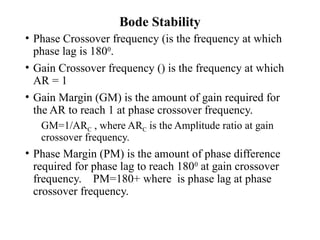
32. Bode Stability
• Phase Crossover frequency (is the frequency at which
phase lag is 1800
.
• Gain Crossover frequency () is the frequency at which
AR = 1
• Gain Margin (GM) is the amount of gain required for
the AR to reach 1 at phase crossover frequency.
GM=1/ARC , where ARC is the Amplitude ratio at gain
crossover frequency.
• Phase Margin (PM) is the amount of phase difference
required for phase lag to reach 1800
at gain crossover
frequency. PM=180+ where is phase lag at phase
crossover frequency.

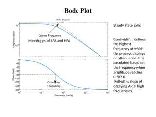
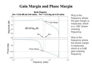
33. Gain Margin and Phase Margin
dB=20 log10AR
Wcg is the
frequency where
the gain margin is
measured, which
is a -180° phase
crossing
frequency.
Wcp is the
frequency where
the phase margin
is measured,
which is a 0-dB
gain crossing
frequency.

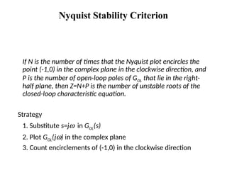
34. Nyquist Stability Criterion
If N is the number of times that the Nyquist plot encircles the
point (-1,0) in the complex plane in the clockwise direction, and
P is the number of open-loop poles of GOL that lie in the right-
half plane, then Z=N+P is the number of unstable roots of the
closed-loop characteristic equation.
Strategy
1. Substitute s=jw in GOL(s)
2. Plot GOL(jw) in the complex plane
3. Count encirclements of (-1,0) in the clockwise direction

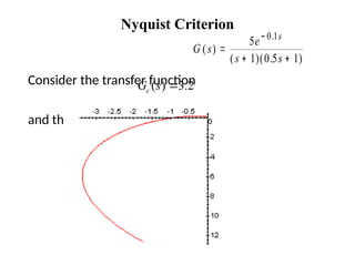
35. Nyquist Criterion
Consider the transfer function
and the P controller
G s
e
s s
s
( )
( )( . )
.

 

5
1 0 5 1
0 1
( ) 3.2
c
G s 