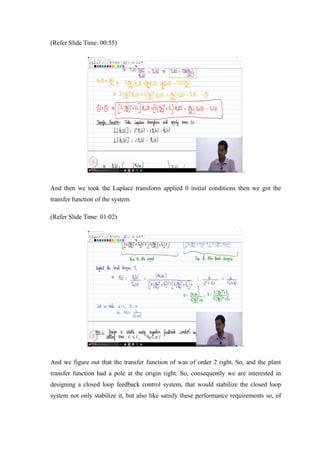
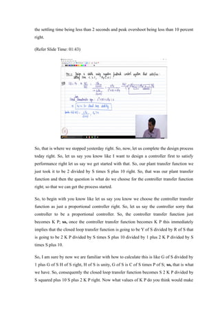
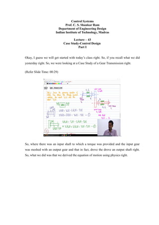
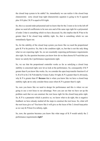
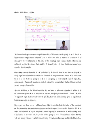
- The document summarizes the process of designing a controller for a gear transmission system to satisfy stability and performance requirements. - It describes deriving the plant transfer function, choosing an initial proportional controller, and analyzing the closed-loop stability and performance using root locus analysis. - Key steps include determining the regions of the real axis on the root locus, identifying asymptotes, and finding a potential breakaway point at -5 where the controller gain is 12.5.

1. Control Systems
Prof. C. S. Shankar Ram
Department of Engineering Design
Indian Institute of Technology, Madras
Lecture – 43
Case Study-Control Design
Part I
Okay, I guess we will get started with today’s class right. So, if you recall what we did
yesterday right. So, we were looking at a Case Study of a Gear Transmission right.
(Refer Slide Time: 00:29)
.
So, where there was an input shaft to which a torque was provided and the input gear
was meshed with an output gear and that in fact, drove the drove an output shaft right.
So, what we did was that we derived the equation of motion using physics right.

2. (Refer Slide Time: 00:55)
.
And then we took the Laplace transform applied 0 initial conditions then we got the
transfer function of the system.
(Refer Slide Time: 01:02)
.
And we figure out that the transfer function of was of order 2 right. So, and the plant
transfer function had a pole at the origin right. So, consequently we are interested in
designing a closed loop feedback control system, that would stabilize the closed loop
system not only stabilize it, but also like satisfy these performance requirements so, of

3. the settling time being less than 2 seconds and peak overshoot being less than 10 percent
right.
(Refer Slide Time: 01:43)
So, that is where we stopped yesterday right. So, now, let us complete the design process
today right. So, let us say you know like I want to design a controller first to satisfy
performance right let us say we get started with that. So, our plant transfer function we
just took it to be 2 divided by S times S plus 10 right. So, that was our plant transfer
function and then the question is what do we choose for the controller transfer function
right; so that we can get the process started.
So, to begin with you know like let us say you know we choose the controller transfer
function as just a proportional controller right. So, let us say the controller sorry that
controller to be a proportional controller. So, the controller transfer function just
becomes K P; so, once the controller transfer function becomes K P this immediately
implies that the closed loop transfer function is going to be Y of S divided by R of S that
is going to be 2 K P divided by S times S plus 10 divided by 1 plus 2 K P divided by S
times S plus 10.
So, I am sure by now we are familiar with how to calculate this is like G of S divided by
1 plus G of S H of S right, H of S is unity, G of S is C of S times P of S; so, that is what
we have. So, consequently the closed loop transfer function becomes S 2 K P divided by
S squared plus 10 S plus 2 K P right. Now what values of K P do you think would make

4. the closed loop system to be stable? So, immediately we can realize it the closed loop
characteristic sorry closed loop right characteristic equation is going to be S squared
plus 10 S plus 2 K P is equal to R 0 right.
So, this is a second order polynomial and we know that for the 2 roots to lie in the left off
plane we need all coefficients to be non zero and of the same sign right for a polynomial
of order 2 that is something which we have discussed. So, this implies that K P has to be
greater than 0 for closed loop stability right. So, that is something which we can
immediately figure out.
So, for the stability of the closed loop system you know like we need the proportional
gain K P to be positive. So, that is the condition right, so, but that is not the only thing
what we are expecting right. So, we are essentially expecting performance requirements
also right. So, the question becomes you know how do we then choose K P such that you
know we satisfy the 2 performance requirements right.
So, we see that the proportional controller works as far as satisfying a closed loop
stability is concerned right; now let us look at the performance. So, consequently if K P
greater than 0 you know like works. So, we consider the open loop transfer function G of
S, H of S to be 2 K P divided by S times S plus 10 right, K P is greater than 0; obviously,
why K P is greater than 0? Because that is when you know like we have a closed loop
stability right, so we only consider those cases where K P is greater than 0, right.
So, now you know like we need to design for performance and this is where we are
going to use a root locus to our advantage. Now you can see that we have set up the
problem such that we can construct the root locus right for the closed loop poles right.
So, K P is a parameter which is positive so, we know what to do right, this is negative
feedback we have already studied all the steps to construct the root locus. So, what will
the root locus give us? You know like it will give us the locus of the 2 closed loop poles
as we vary K P from 0 to infinity, right.
So, now, the question becomes you know like what range of K P would satisfy the 2
performance requirements right?

5. (Refer Slide Time: 06:47)
.
So, if you look at the performance requirements you know like the settling time being
less than 4 seconds you know like if you compare it with that of an under damped second
order system; that means, 4 zeta 4 by zeta omega n should be less than 4 or zeta omega, n
should be greater than 1 or in a sense you know like we can say that look you know like I
want the real part of the pole to be less than minus 1. So, we wanted 2 seconds right
sorry about that. So, we wanted 2 so, zeta omega n should be greater than 2 and minus
zeta omega n should be less than minus 2 am I correct?
So, that is what which we chose in this particular problem. So, then if you recall
maximum peak overshoot less than 10 percent, we have already done a problem right.
So, where we did this and that gave a constraint on zeta right and then it once again get
led to a constraint on the angle beta, do you remember? Can you tell me what was that
was we already did this problem, right?
So, M P less than 10 percent means you know like please recall e power minus zeta pi
divided by square root of 1 minus zeta squared should be less than 0.1, right. So, this
gave us zeta should be greater than I think if I recall vaguely it was around 0.591 or
something like that right. So, this implied that the angle beta should be less than some
53.76 degrees right that is what we had.
So, that is how we can convert the performance specifications into regions in the closed
loop plane sorry regions in the S plane that we want. So, let me draw the S plane and

6. then we will start plotting these regions. So, let us this is the real axis, this is the
imaginary axis, this is a s plane, this is the origin.
Now, let me draw the 2 desired regions. So, let us say this is minus 2. So, what happens
is a if I draw a vertical line at minus 2, so, that gives me the boundary for settling time
performance, then if I draw 2 lines, but that make an angle of 53.76 degrees right. This
angle is 53.76 degrees that gives me the condition on peak overshoot right. So, this is
something which you already discussed.
So, the net feasible area, then comes out to be you know like let me draw it in a different
color, let us say we choose green. So, the net feasible a region for us that will satisfy both
performance conditions will be this open trapezoidal region right. So, whose boundary I
am drawing in green color, so that is what it is. So, that is where I want our closed loop
poles to be. Now let us figure out what values of K p would do this job alright, so, that is
what we want to do right.
So, let us start our analysis right. So, our open loop transfer function is this right 2 K p
divided by S times S plus 10 right. So, let us start constructing the root locus right. So,
let us construct the root locus. So, step 1, what is the first step? You locate the open loop
poles and open loop zeros in the S plane right. So, where are the open loop poles? There
is one open loop pole at the origin and let us say this is let us say you know that is really
minus 10, but let me extend it a little bit.
So, let us say I mark minus 10 here, so, minus 10 here yes right. So, consequently the
value of n is 2, the value of m is 0, there are 2 open loop poles at 0 and minus 10, there
are no open loop zeros right. So, correct so, that is a first step. So, please remember our
open loop transfer function let me write it here once again on top, G of S, H of S is going
to be 2 K p divided by S times S plus 10.
Of course we are considering K p to be positive right because that condition came from
closed loop stability right requirement of closed loop stability. So, let us go to the next
step.

7. (Refer Slide Time: 12:40)
.
So, what is the next step? So, step 2 is to determine the regions of the root locus sorry the
regions of the real axis that lie on the root locus. So, for that you know like let us look at
the real axis, we can immediately see that the real axis is divided into 3 regions minus
infinity to minus 10 or minus 10 to 0 and 0 to infinity right.
So, now what is the test that we need to adopt you choose a test point in any of the one of
the regions, look to the right of the test point. The number of real open loop poles and
real open loop 0’s should be odd right. So, if you take a test point in the region minus
infinity to minus 10 you look to the right, let us say you take a test point here let us say
we call it as S t 1 and you look to the right how many real open loop poles and open loop
zeros do we have? We have 2, right that is an even number. So, this region does not lie
on the root locus.
Now, if we repeat considering a test point in the region minus 10 to 0, take a test point
and look to the right you have 1, open loop pole on the real axis right to the right. So,
that is going to be odd right. So, let us say you take a test point somewhere here
wherever we want right. So, and you look to the right, you see that there we have 1 real
open loop pole to the right that is an odd number.
So, minus 10 to 0 will lie on the root locus. Then we take a test point in between 0 to
infinity, let us say we call it as S t 3 you look to the right there are none right. So, there
are no open loop poles or no loop poles zeros to the right on the real axis of the any test

8. point in this region. So, the only region of the real axis that lies on the root locus is the 1
between minus 10 and 0. So, that is what we have right as a second step, is it clear?
So, then we move to the next step. So, what is step 3? Step 3 is essentially figuring out
asymptotes right. So, we are going to have n minus m which are essentially 2, which is
the number is 2 here. So, there are going to be 2 asymptotes right in this particular
problem. So, the angle of the asymptotes or the angle made by the asymptotes right with
the real axis is going to be plus or minus 180 degrees times 2 k plus 1 divided by n minus
m alright, so that is what we have.
So, in this case since n minus m is 2. So, we can immediately see that this is going to be
plus or minus 90 or we can write it as 90 degrees and 270 degrees. So, depending on how
we want to write so, that is what we want to have. And not only angle, but also the point
of intersection of the asymptotes is something which we need to calculate.
So, the point of intersection of the asymptotes that is going to be sum of open loop poles
minus sum of open loop zeros divided by n minus m right. So, open loop poles the sum
is going to be 0 1 minus 10 and open loop zeroes there are none. So, divided by n minus
m which is 2 and the number happens to be minus 5 alright that is that is going to be the
point of intersection of the asymptotes right.
So, let us go here so, let me just erase all these things, I think I am sorry about that. So,
let us just go and go mark these things right. So, let us say minus 5 is somewhere here.
So, what is going to happen is it the there are going to be two asymptotes, one is going to
just go at plus 90 alright all the way up and one is going to go at 270 degrees or minus
90. So, those are the 2 asymptotes right as k tends to infinity. So, as k tends to or K p
tending to infinity this is the direction in which the root locus branches would be going
alright will tend to once. So, that is that is step 3 of the construction of the root locus.
So, then let us go to step 4. So, what is step 4? We have to figure out whether there are
any breakaway or a breaking points right. So, how do we figure out whether there are
any breakaway or breaking points, we look at the open loop transfer function.

9. (Refer Slide Time: 18:04)
.
So, immediately you see that the polynomial A of S in this case is going to be 2, that is it
right because why? Please note that G of S, H of S we need to write it as K times A of S
divided by B of S of course, in this time in this case K p right because that is what we are
calling it as. So, K p times 2 divided by S times S plus 10, right that is our open loop
transfer function right.
Open loop transfer function is 2 K p divided by S times S plus 10, we have to keep K p
away right because the structure is the constant or the parameter K times A of S divided
by B of S. So, A of S is going to be 2, B of S is going to be S times S plus 10 right. So,
consequently A prime S is going to be 0, B prime S is going to be 2 S plus 10 that is what
we are going to have right.
So, this will lead to the following right. So, we need to solve the equation A prime S, B
of S minus B prime S, A of S equals 0. So, this will just give us minus 2 times 2 S plus
10 equals 0 right that is what we will get. So, this will immediately give as a potential
break away point at minus 5.
So, we are not done yet as I told you know like we need to find the value of the constant
or the parameter not constant the parameter in the open loop transfer function this K p
here. So, the value of K p at S equals S b that is going to be minus B of S divided by A of
S evaluated at S equals S b. So, what is this going to be if you substitute minus 5? We
will get minus 5 times 5 right, S times S plus 10 right, am I correct and divided by 2. So,

10. this will come to be 12.5 and that is greater than, right. So, this implies that S b equals
minus 5 is a breakaway point. Why am I calling it as a breakaway point? Once again it is
a pretty simple by now right.
So, please note that see for example, let us say you know like I am plotting the final root
locus let us say in red. So, please note that one branch will start from this open loop pole
at minus 10 and it will start traveling to the right, why because the left it can go to the
left right as we know from step 2 and similarly another branch will start from the open
loop pole at 0 and start traveling to the towards the left and obviously, these 2 things
come and meet at minus 5. So, minus 5 becomes a breakaway point where K p is 12.5.
So, that is what we have as a breakaway point yes.
Student: (Refer Time: 21:43).
May occur, may not occur. So, it depends on the problem. So, if you have alternating
poles and 0’s, but if you have complex conjugate open loop poles right and depending on
the relative order of the system values of n and m you may have asymptotes going on the
real axis right. So, you may have, but if you have open loop 0, certainly some of the
branches will terminate at the open loop 0 has K tends to infinity. So, that is something
which we need to it really depends on the problem under consideration.
See another reason is that like, why I am doing only like problem still order 2 in class is
because of the algebra. See if I can construct a higher order system to essentially
demonstrate your points, but then like you will see that the computations will become
complex right. Here my primary purpose is to introduce the concepts to you, so, that like
and also we work it out using simple problems to begin with and as you go along you
will see that the problems will become tougher and tougher in your homework you may
get tougher problems for which you can make use of the help of some computational
tools also that is fine right.
So, but there can be various cases yeah.
Student: (Refer Time: 23:10).
You mean the breakaway point?
Student: Yes sir.

11. So, if you have a, what you say breakaway point in the complex plane still you need to
check the value of K. If you have K to be positive, then it is a potential breakaway point
right or breaking point but then there we need to remember one thing right if you have a
complex root the conjugate also must be a root.
So, we are talking about a very complex situation you know like where you have
branches just intersecting in the complex plane right and then like going away. Let me
maybe construct an example for that and then like show it to you right yeah, but yeah I
think maybe I will construct a transfer function and give it to you, maybe you can use
math lab to construct the root locus and see for yourself.
Student: Sir, what is the meaning of break away (Refer Time: 24:05).
See you may have 2 root low side branches coming and intersecting at some point in the
complex plane you can have it right. So, there is nothing which says we cannot right, but
the only catch is it as I told you know like if you have a breakaway point or breaking
point in the complex where that is which is complex right, the conjugate also must be 1
right, but the condition is that like K should be still positive, of course, if you are
considering positive K right or negative if you are considering negative K that constraint
we need to always check yeah.