Download as PPSX, PPTX

![State-Space Equations
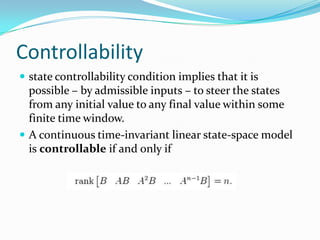
• In a state-space system representation, we have a system of two equations
• equation for determining the state of the system
x'(t) = g[t0,t,x(t),x(0),u(t)]
• equation for determining the output of the system
y(t) = h[t,x(t),u(t)]
• x‘(t) = A(t)x(t) + Bu(t)
• y(t) = C(t)x(t) + Du(t)](https://image.slidesharecdn.com/aalokganeshsujhit-120309114857-phpapp01/85/linear-algebra-in-control-systems-18-320.jpg)


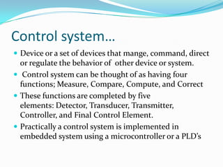
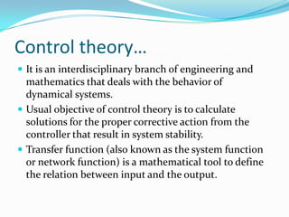
This document discusses control systems and their analysis using state space models. It defines the key components of a control system and explains how state space representation models systems using state variables and matrices. The document also covers analyzing stability, controllability and observability of state space models.