Downloaded 55 times


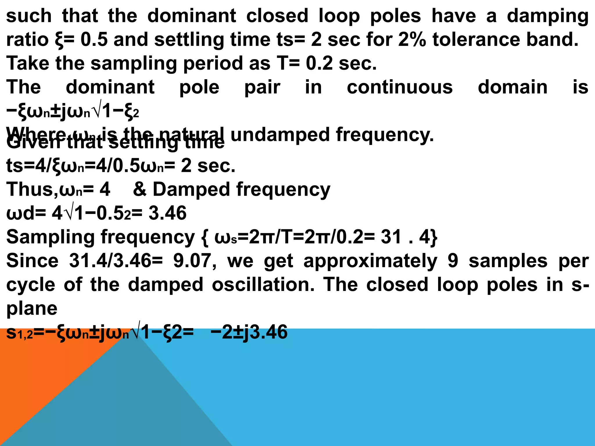
![Thus the closed loop poles in z-plane
z1,2=exp(T(−2±j3.46))
|z|=e−T ξ ωn=exp(−0.4) = 0.676
<z=Tωd= 0.2×3.464 = 0.69 rad = 39.690
Thus,
z1,2= 0.67639.70∼=0.52±j0.43
G(z) =Z[(1−e−0.2s/s)*1/s(s+ 1)]=
(1−z−1)Z[1/s2(s+ 1)]∼=0.02(z+ 0.93)/(z−1)(z−0.82)](https://image.slidesharecdn.com/designofsampleddatacontrolsystems5thlecture-181106183900/75/Design-of-sampled-data-control-systems-5th-lecture-15-2048.jpg)


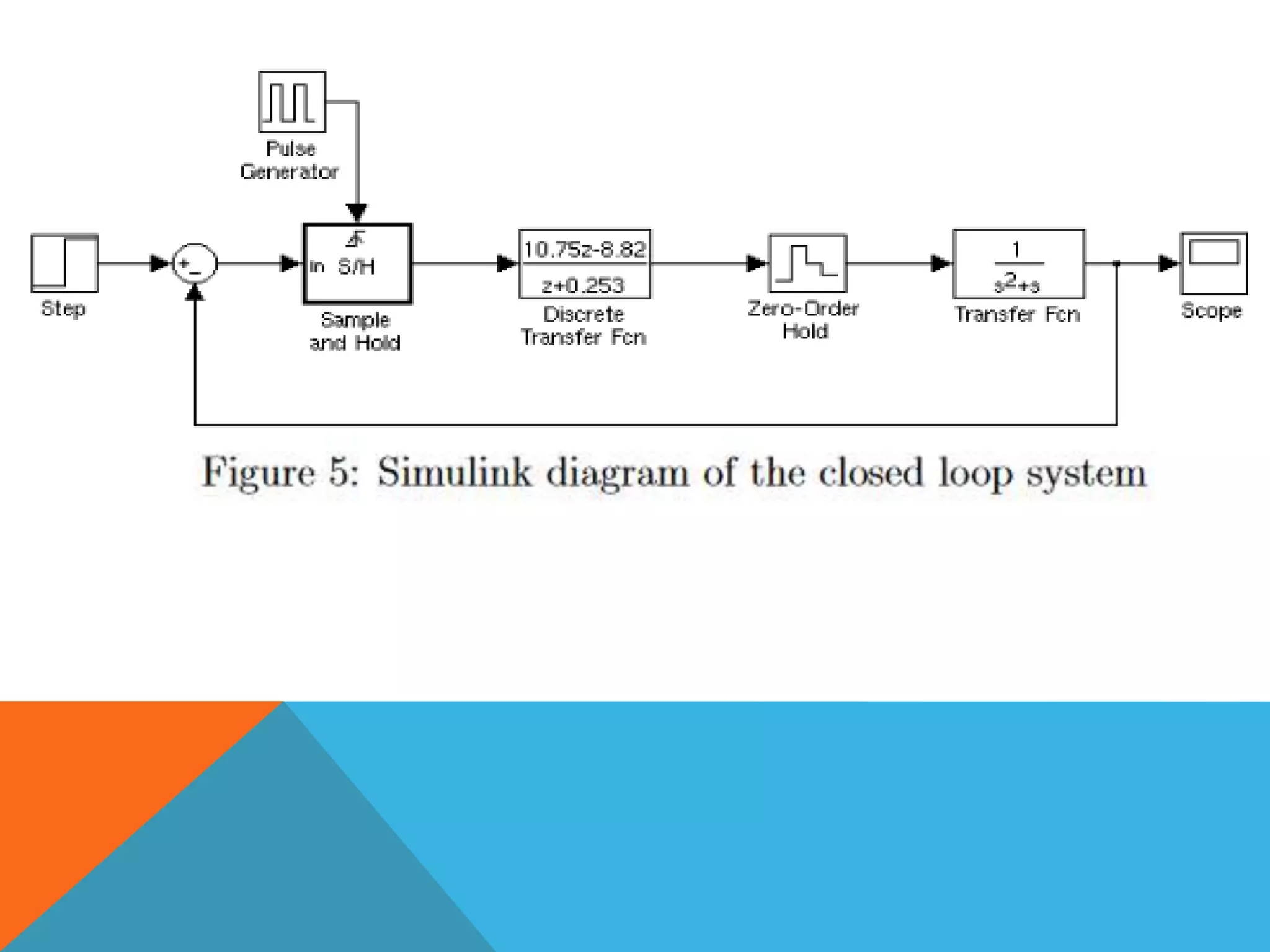
![Example 2
First order type 1 system with loop gain
L(z)=1/Z−1
•Obtain the root locus plot.
•Obtain the critical gain.
The solution in Matlab will be
>> num=[0 0 1];
>> den=[0 1 -1];
>> h=tf(num,den);
>> sys_d=tf(num,den,-1);
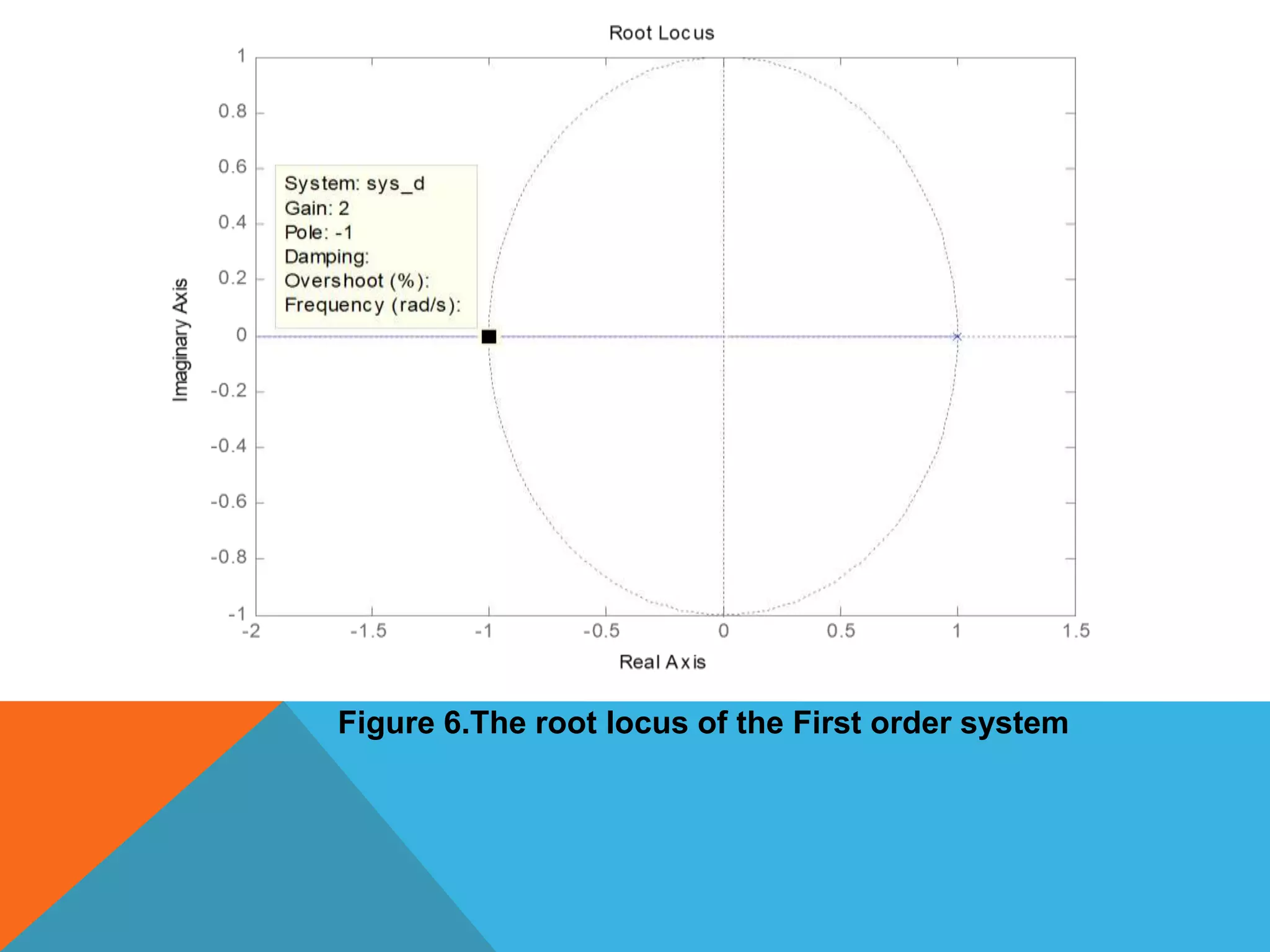
>> rlocus(sys_d);](https://image.slidesharecdn.com/designofsampleddatacontrolsystems5thlecture-181106183900/75/Design-of-sampled-data-control-systems-5th-lecture-26-2048.jpg)
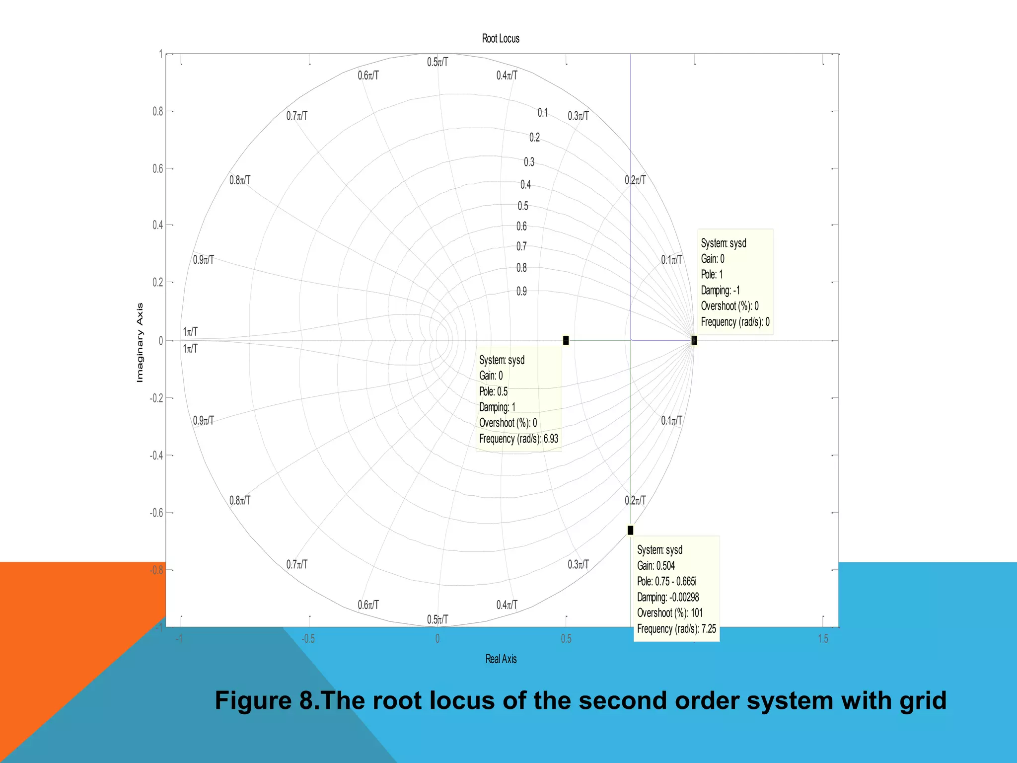
![First the example can be solved directly by Matlab software
as follows
>> g=tf(num, den, T) % sampling period T
>> rlocus(g) % Root locus plot
>> zgrid(zeta, wn) % Plot contours
% zeta= vector of damping ratios
% wn = vector of undamped natural
% frequencies>> num=[0 0 1];
>> den=[1 -1.5 0.5];
>> h=tf(num,den,0.1);
>> sysd=tf(num,den,0.1);
>> rlocus(sysd);
>>zgrid;
>>axis equal;](https://image.slidesharecdn.com/designofsampleddatacontrolsystems5thlecture-181106183900/75/Design-of-sampled-data-control-systems-5th-lecture-29-2048.jpg)

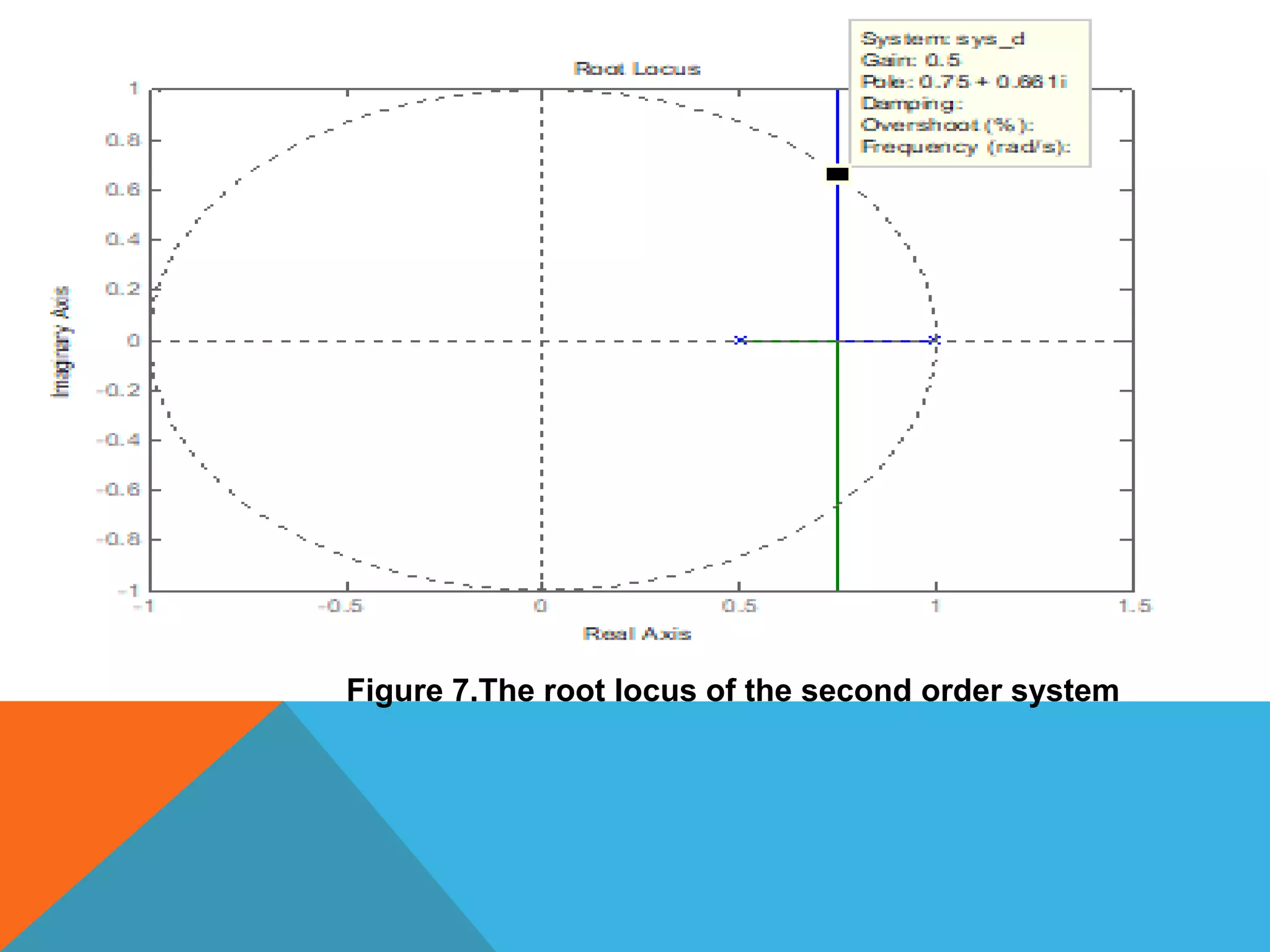
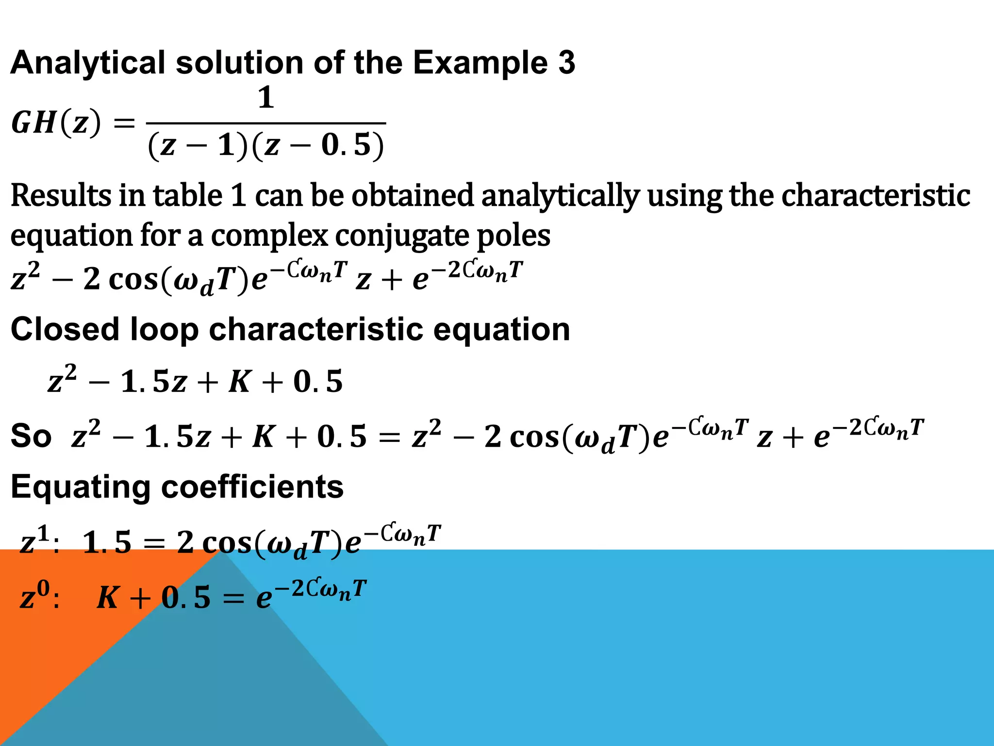


This document discusses the design of digital controllers using root locus analysis. It provides examples of designing proportional controllers for first and second order systems to meet specifications on damping ratio, natural frequency, and settling time. The procedures involve constructing root loci, determining breakaway points and critical gains, and using the MATLAB root locus tool to plot contours and obtain design values for proportional gain.
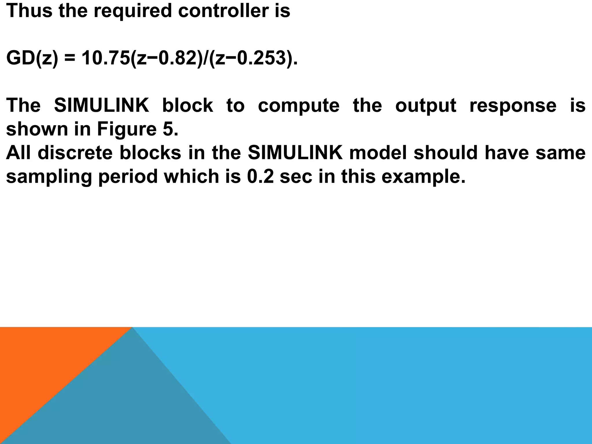
Introduction of Assist. Prof. Dr. Khalaf S. Gaeid from Tikrit University, focusing on designed sampled data control systems.
Overview of key contents including: Root Locus, construction rules, controller types, pole-zero cancellation, design procedure, Simulink implementation, and assignments.
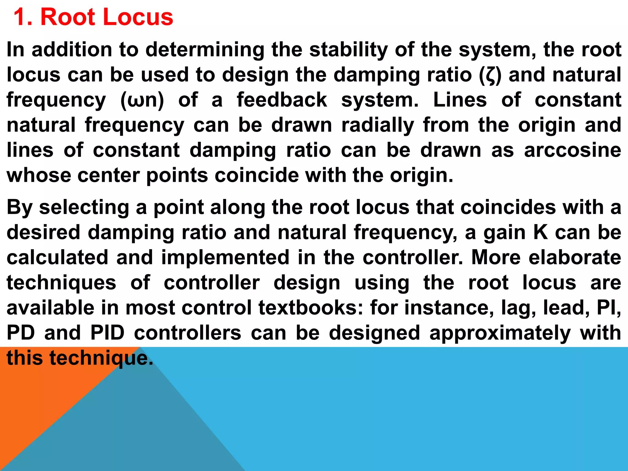
Root locus helps determine system stability, damping ratio (ζ), and natural frequency (ωn) for feedback systems.
Discusses sensitivity of system roots and the integration of root locus with the Routh-Hurwitz criterion for stability assessment.
Construction rules include symmetry about the real axis, branches starting from poles, and conditions for the real-axis portions being part of the root locus.
Calculates asymptotes for the root locus and defines breakaway points and the calculations required for angles of departure and arrival.
Introduces various controller types (PI, PD, PID) and their effects on system performance, steady state response, and stability.
Explains pole-zero cancellation in controller design, including risks of using unstable poles and the importance of careful placement of poles and zeros.
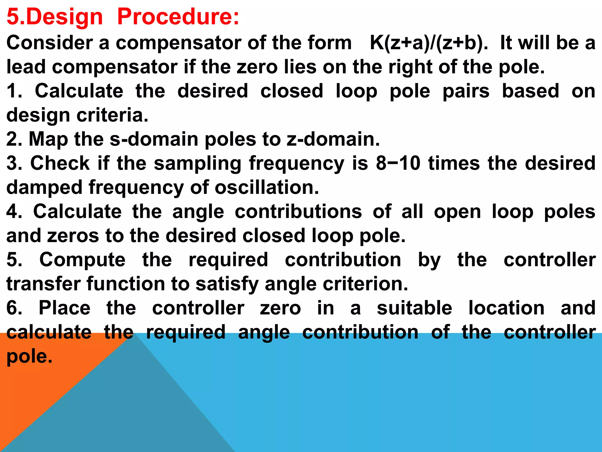
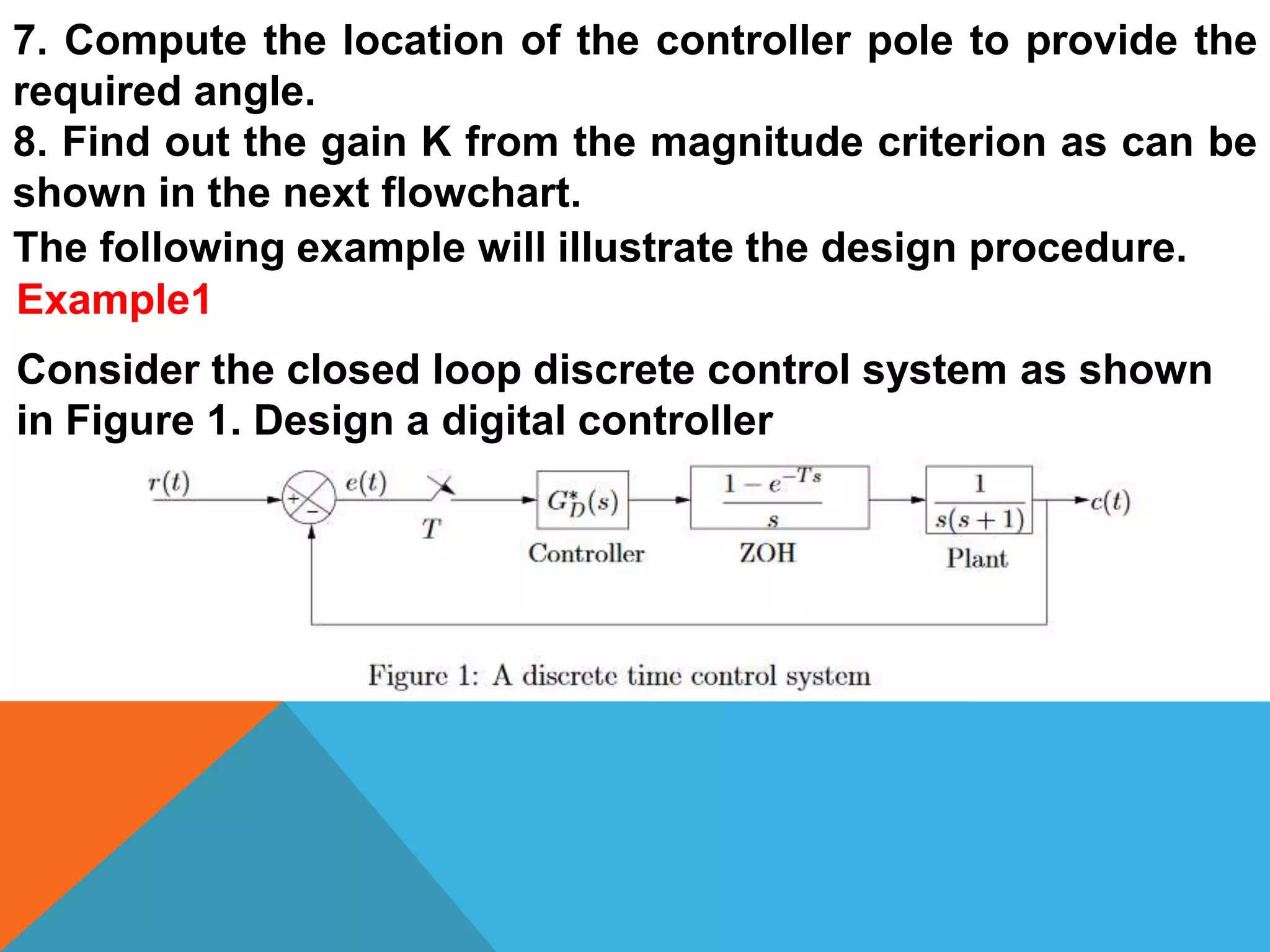
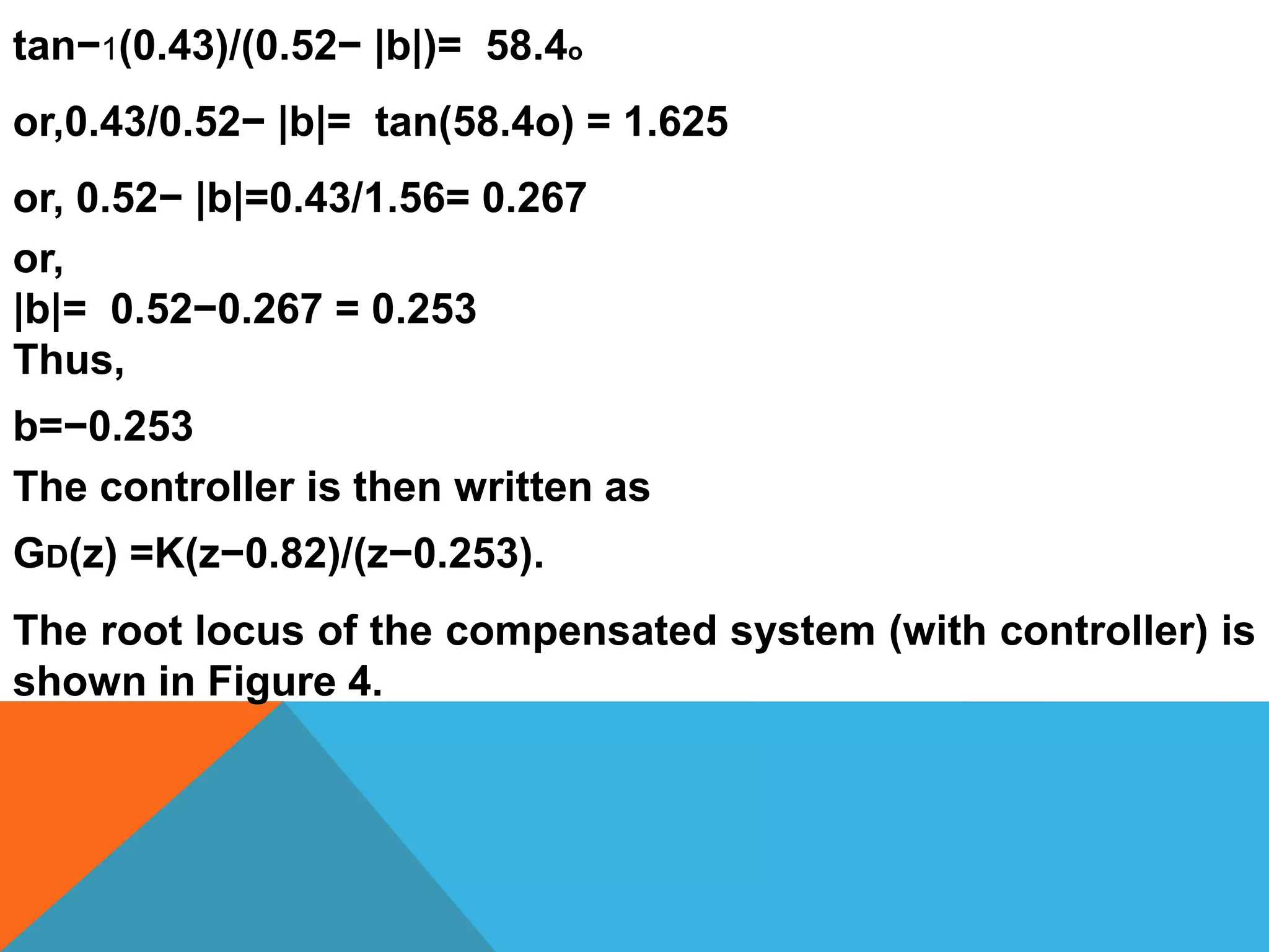
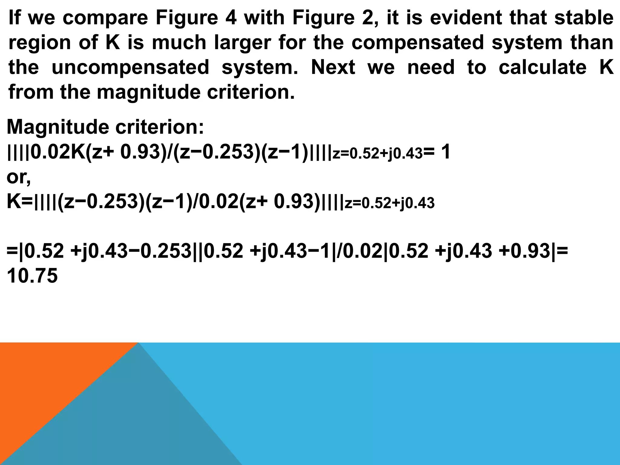
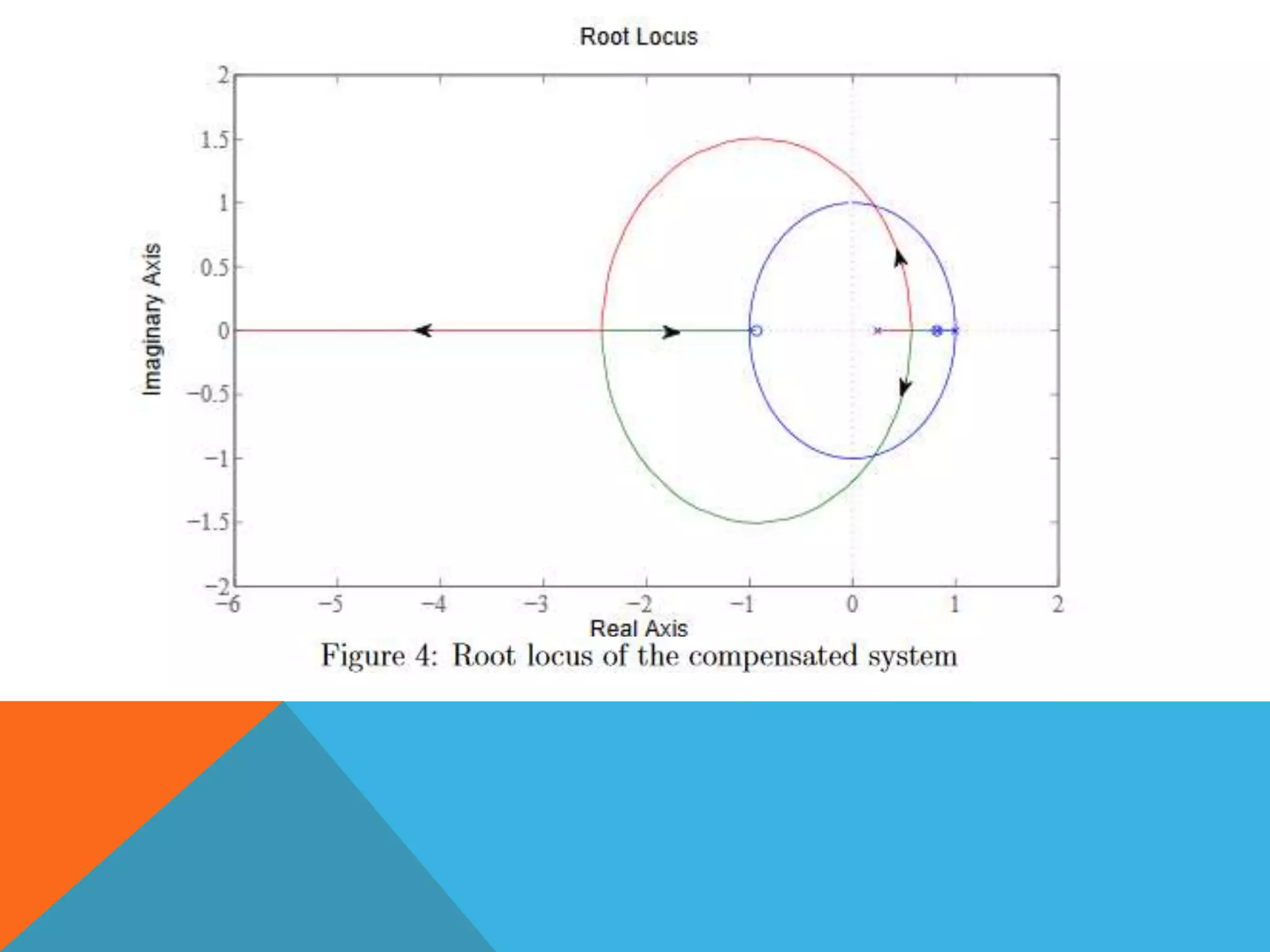
Detailed stepwise approach for designing a compensator and verifying closed loop pole location and angle contributions.
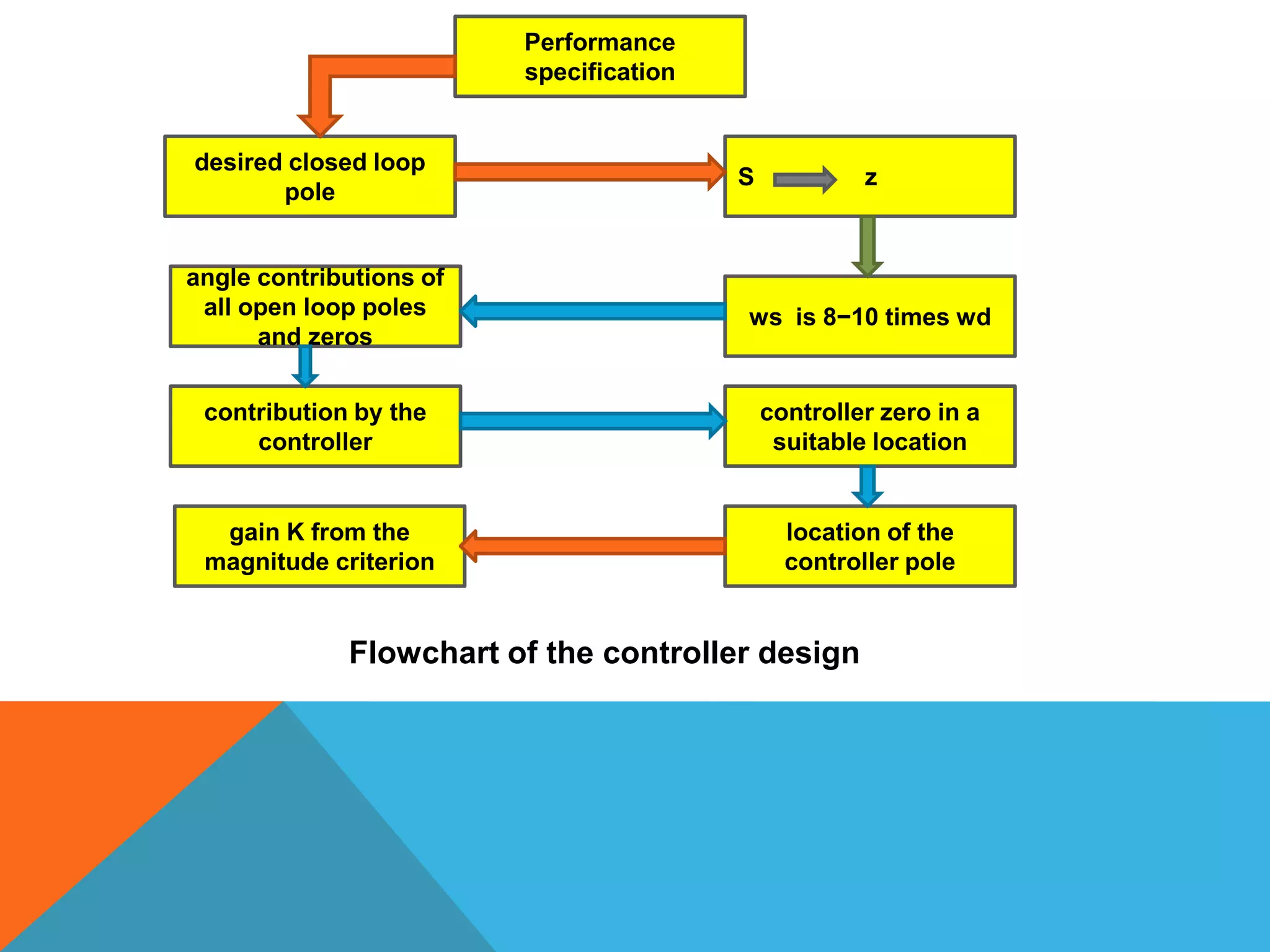
Provides an illustration of digital controller design processes with flowchart representation and example calculations.
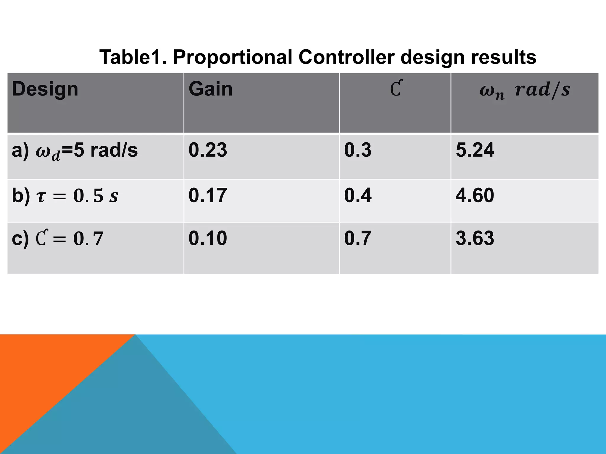
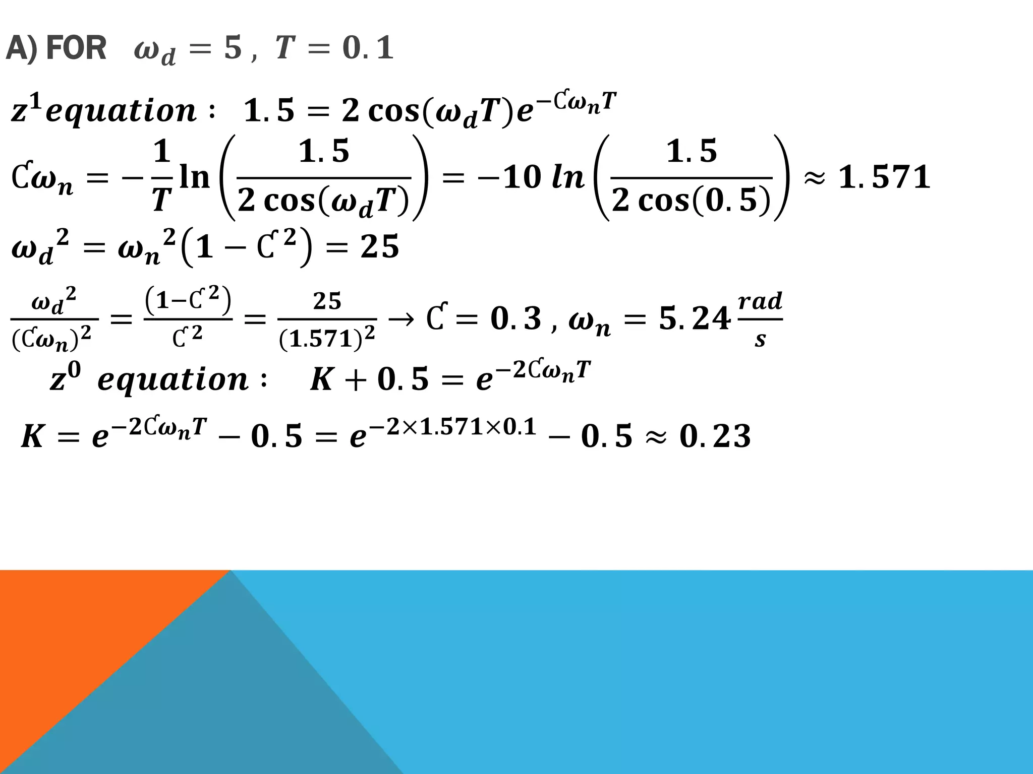
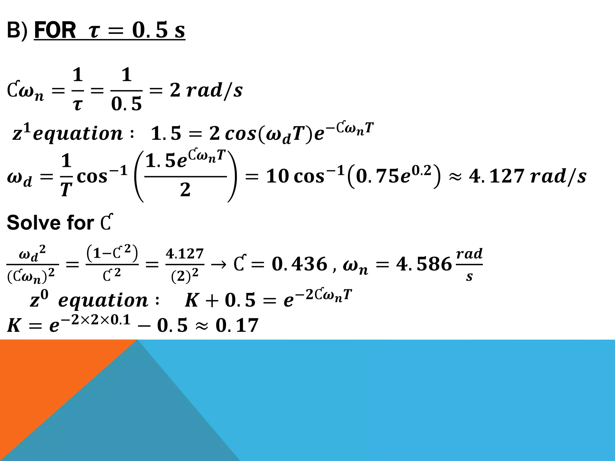
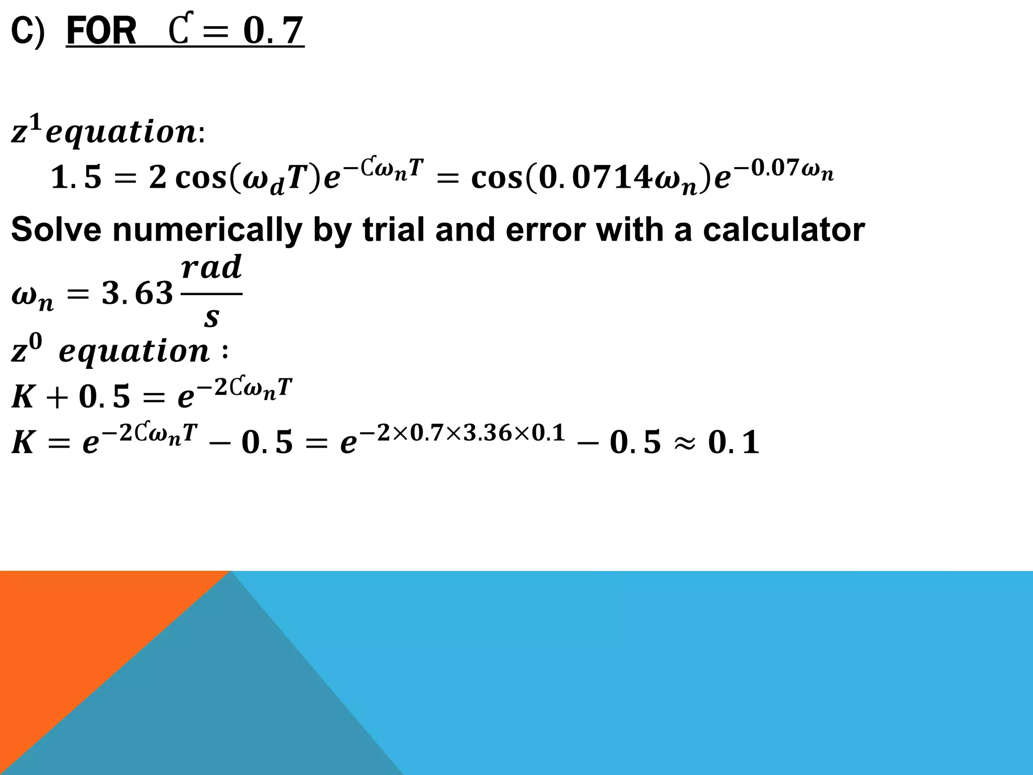
Details setup for controller designs aiming for specific performance such as settling times and frequency analysis.
Calculates closed loop poles in z-plane from given damping ratios, settling times, and their corresponding expressions.
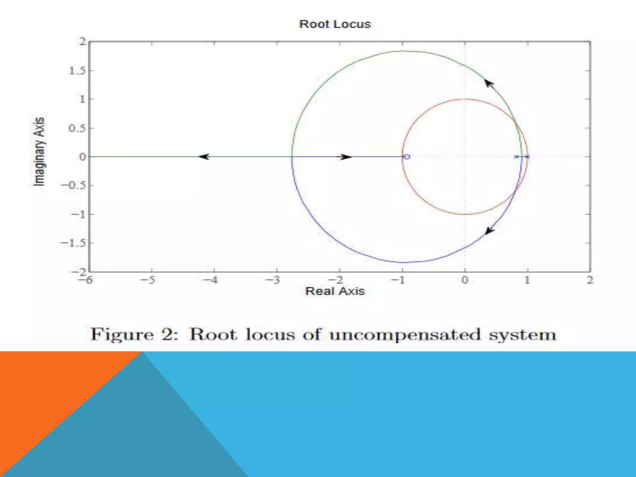
Discussion on the root locus of the uncompensated system and its stability characteristics.
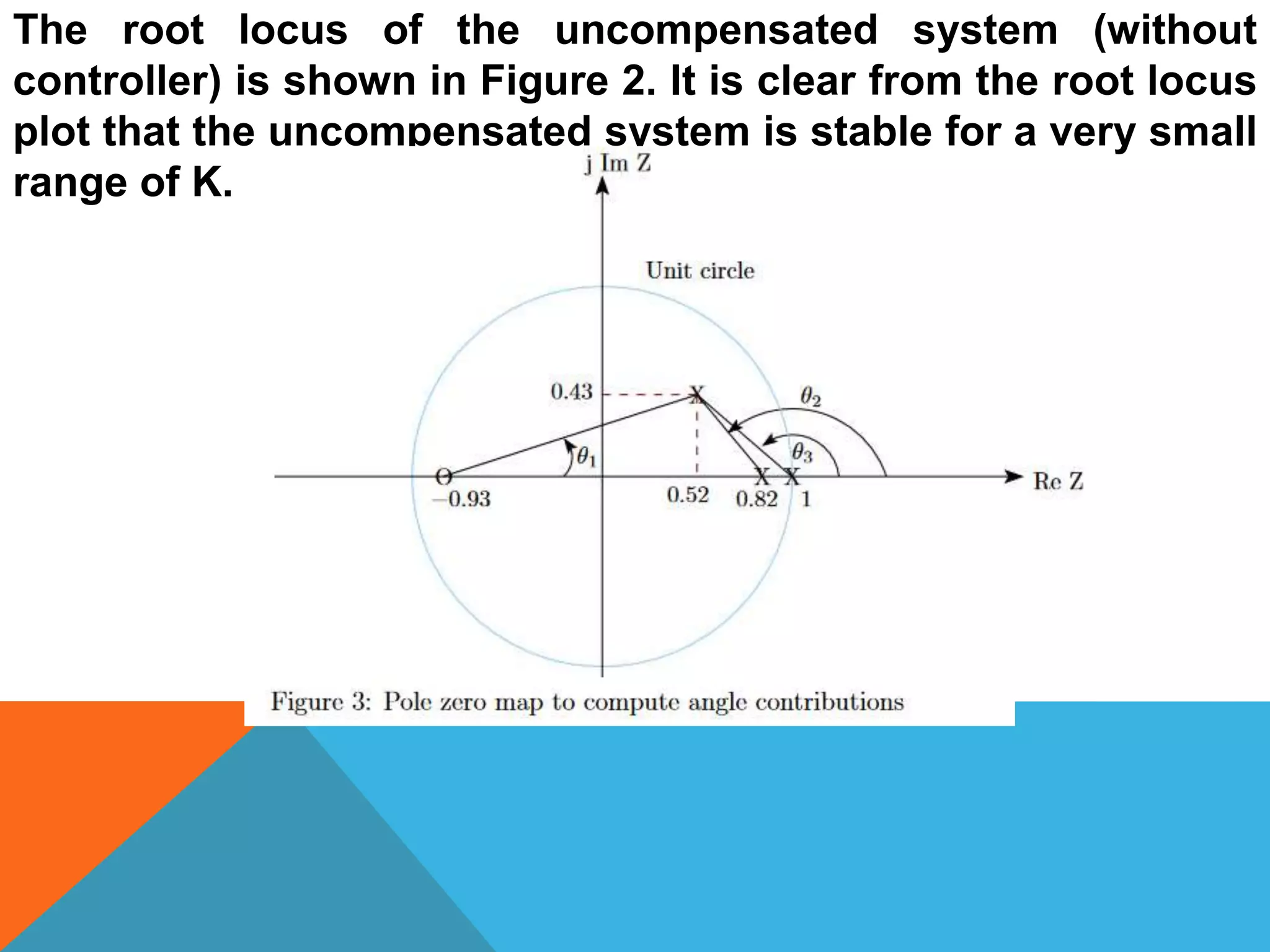
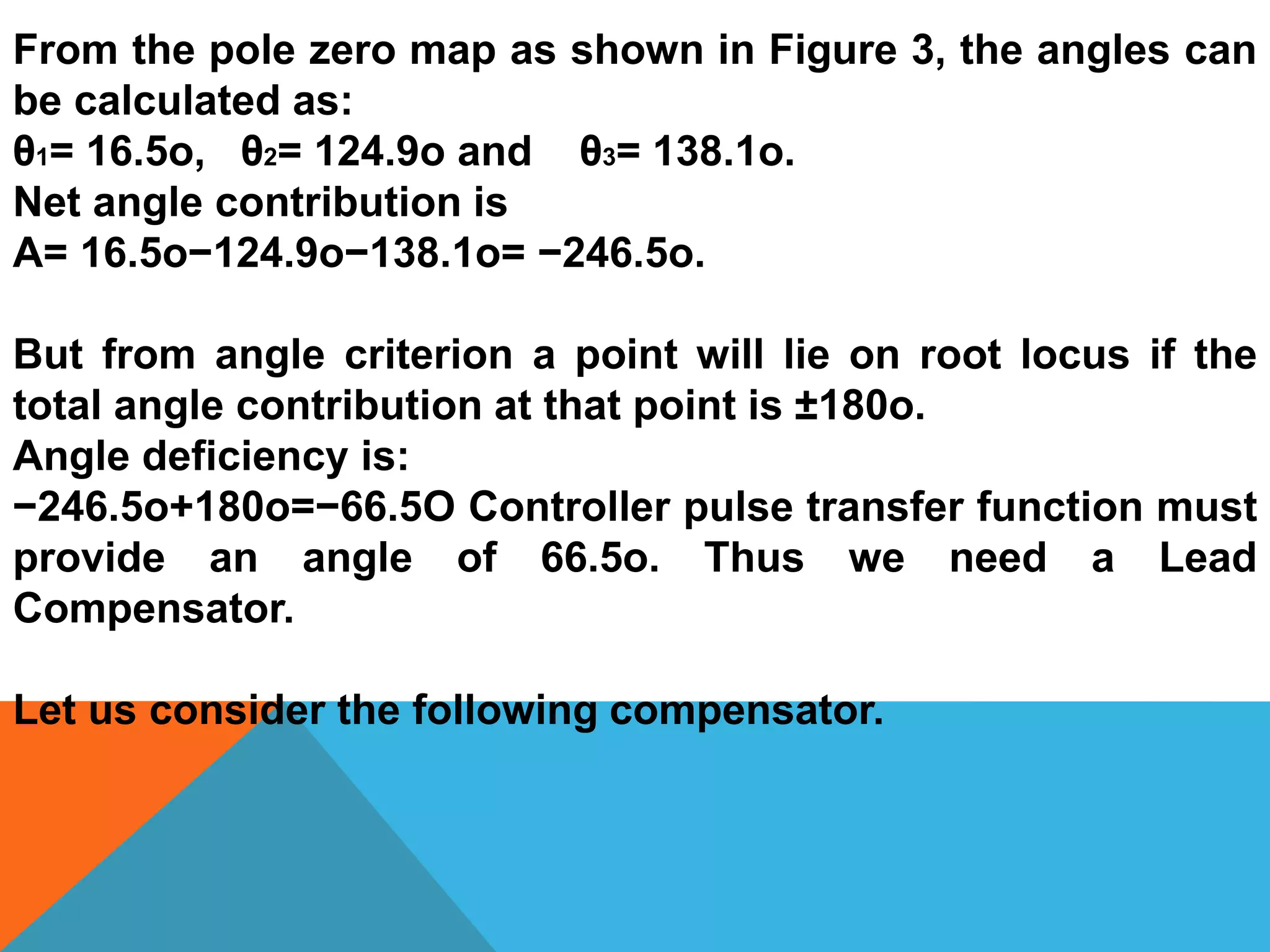
Analyzes angle contributions in pole-zero maps for determining the overall root locus configuration.
Step-by-step construction of a lead compensator and adjustments for achieving desired angle contributions.
Demonstrates how to obtain root locus plots and critical gains using MATLAB for different systems.
Describes numerical methods and MATLAB commands used for stability analysis and gain calculations.
Details analytical solutions based on closed loop characteristic equations, providing further insights into system dynamics.
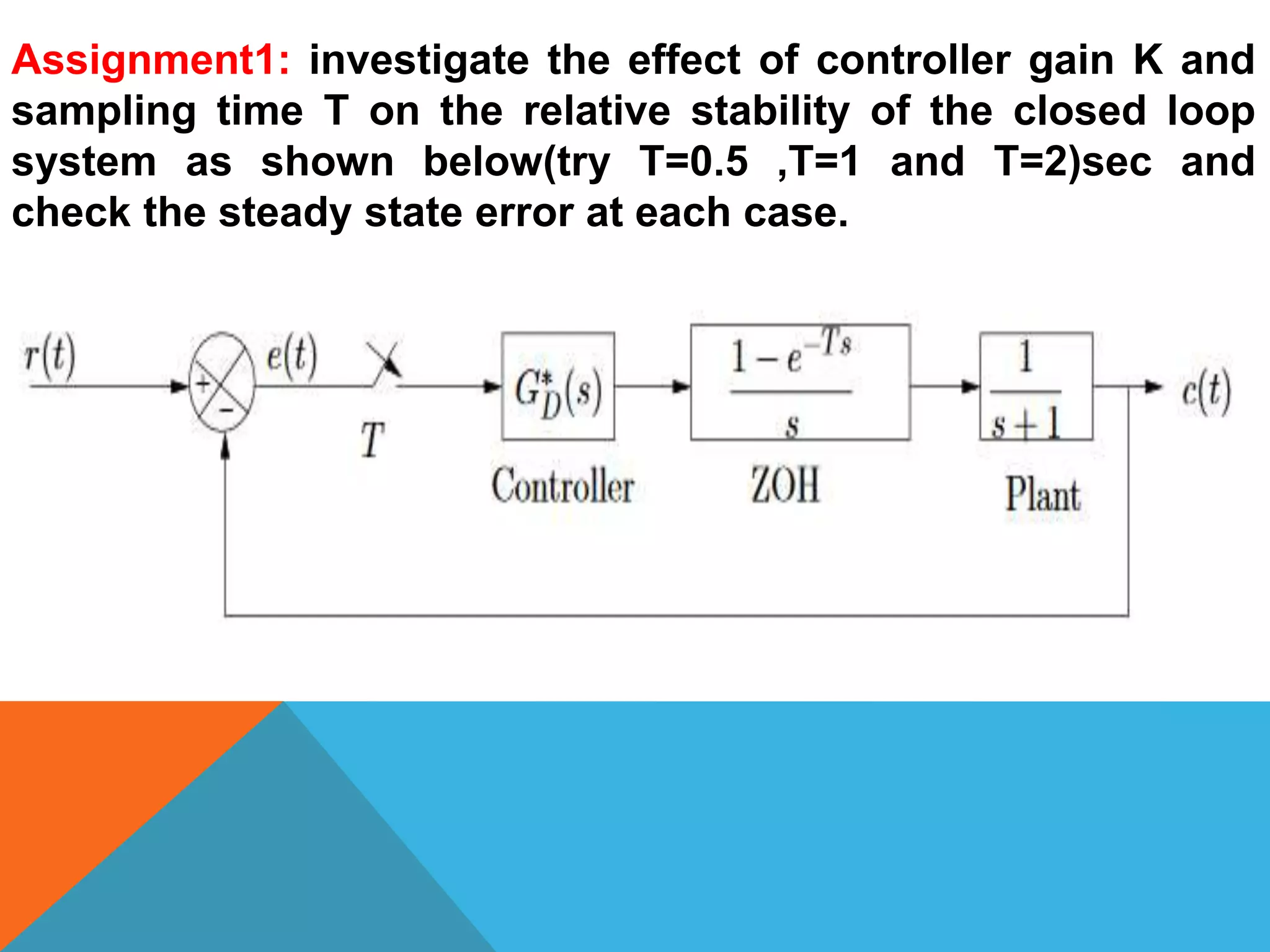
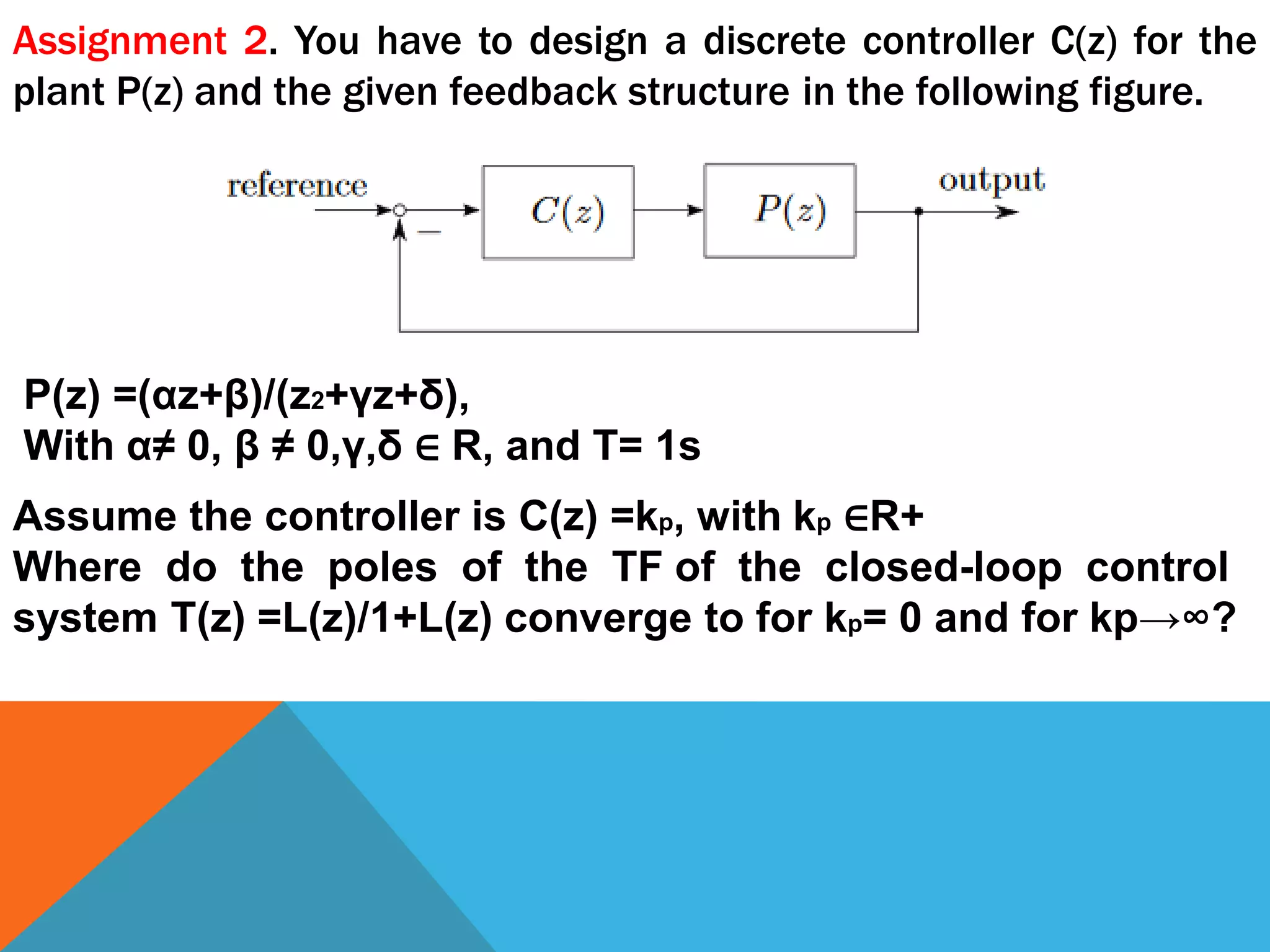
Presents assignments for students related to controller gain effects and design of discrete controllers.
Thanks and closing remarks on the topic of sampled data control system design.


![Digital Signal Processing[ECEG-3171]-L00](https://cdn.slidesharecdn.com/ss_thumbnails/dspl00-180427094421-thumbnail.jpg?width=640&height=640&fit=bounds)