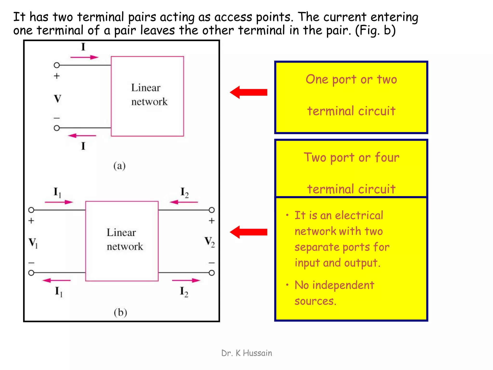
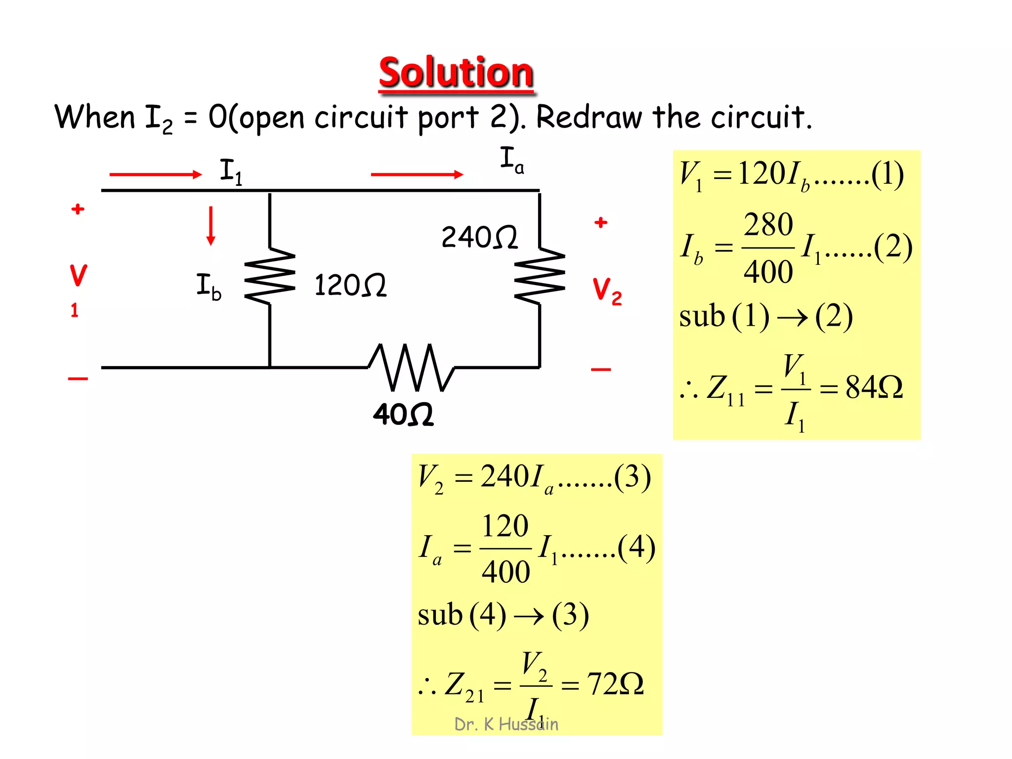
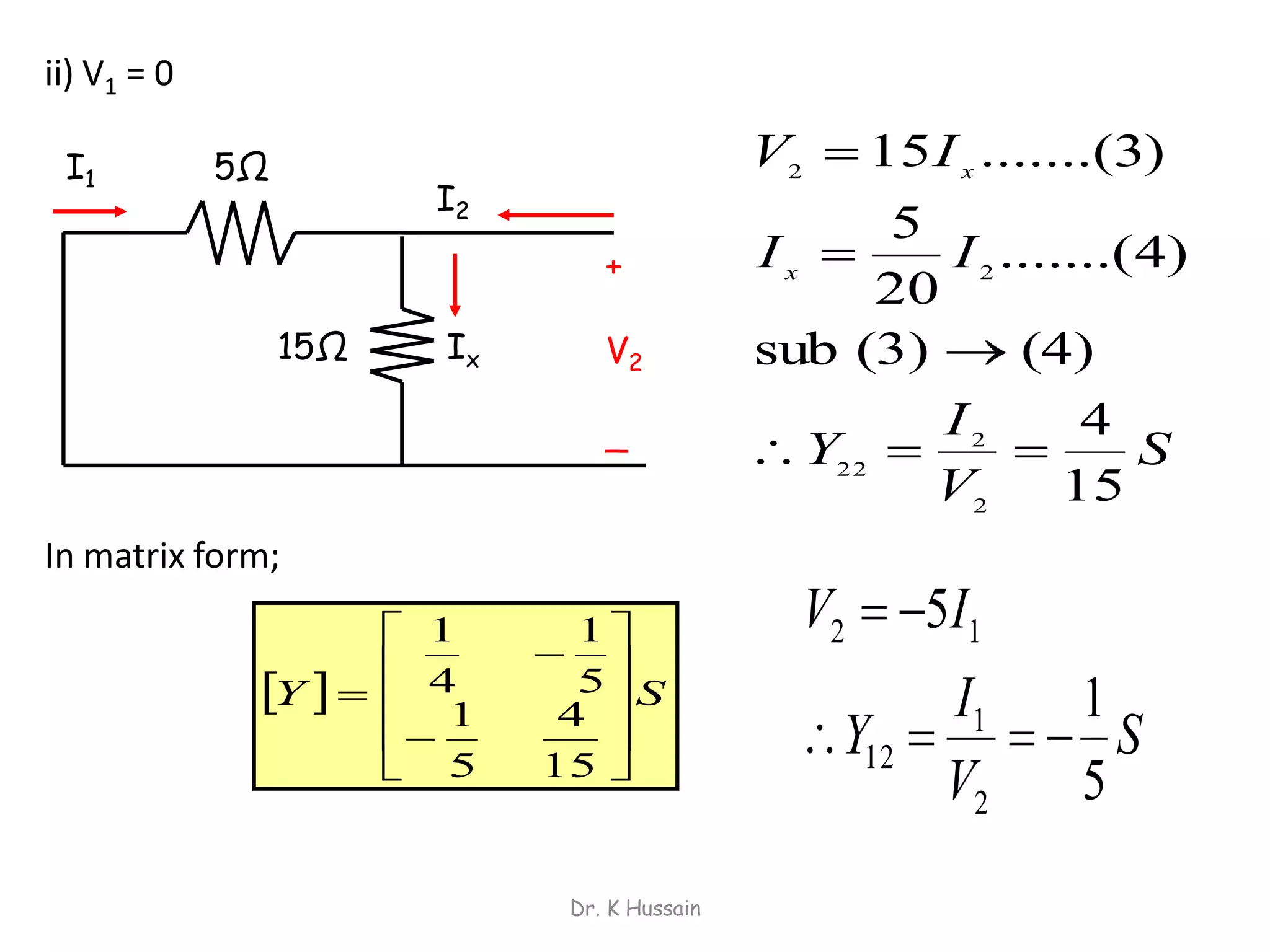
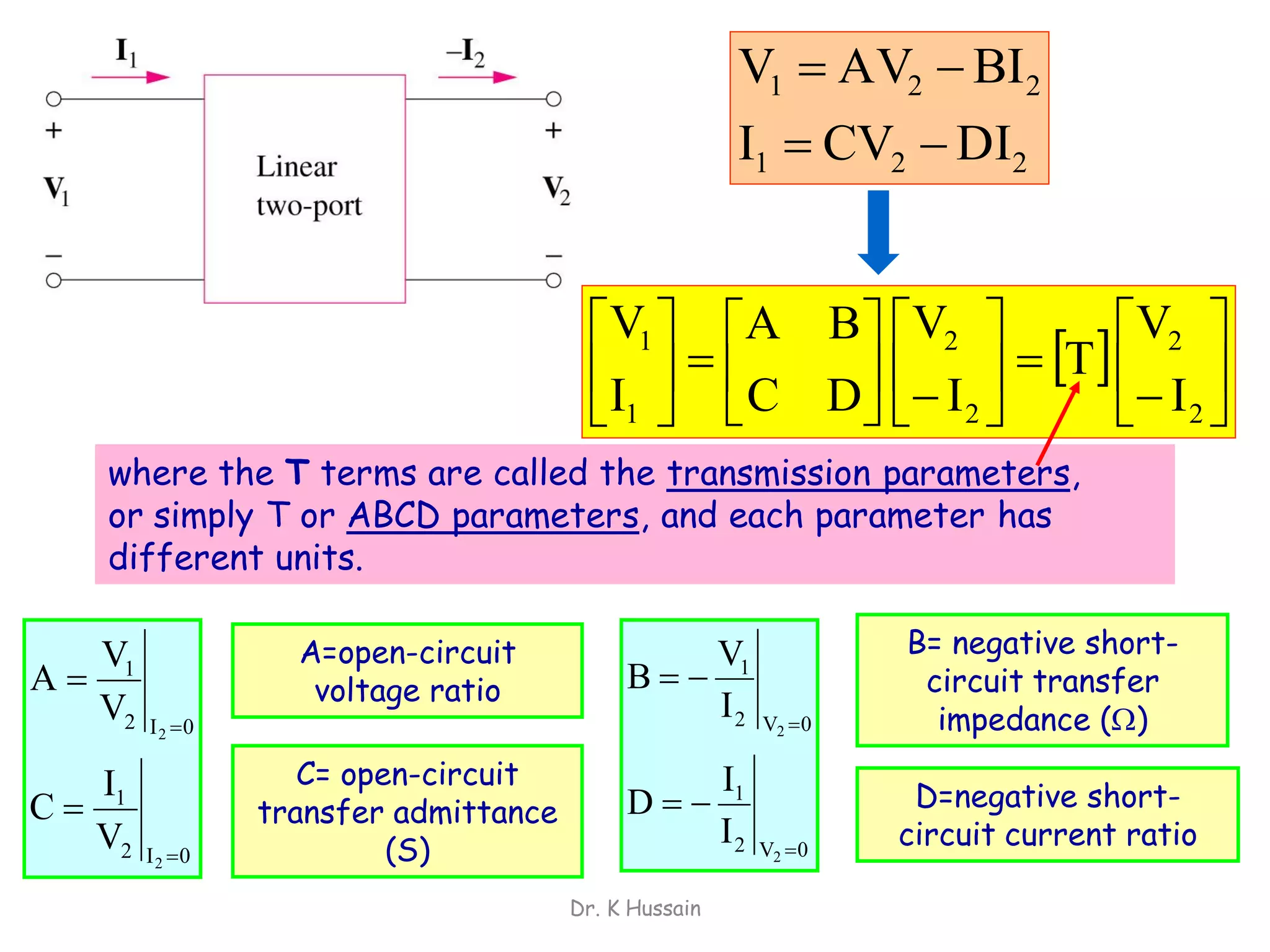
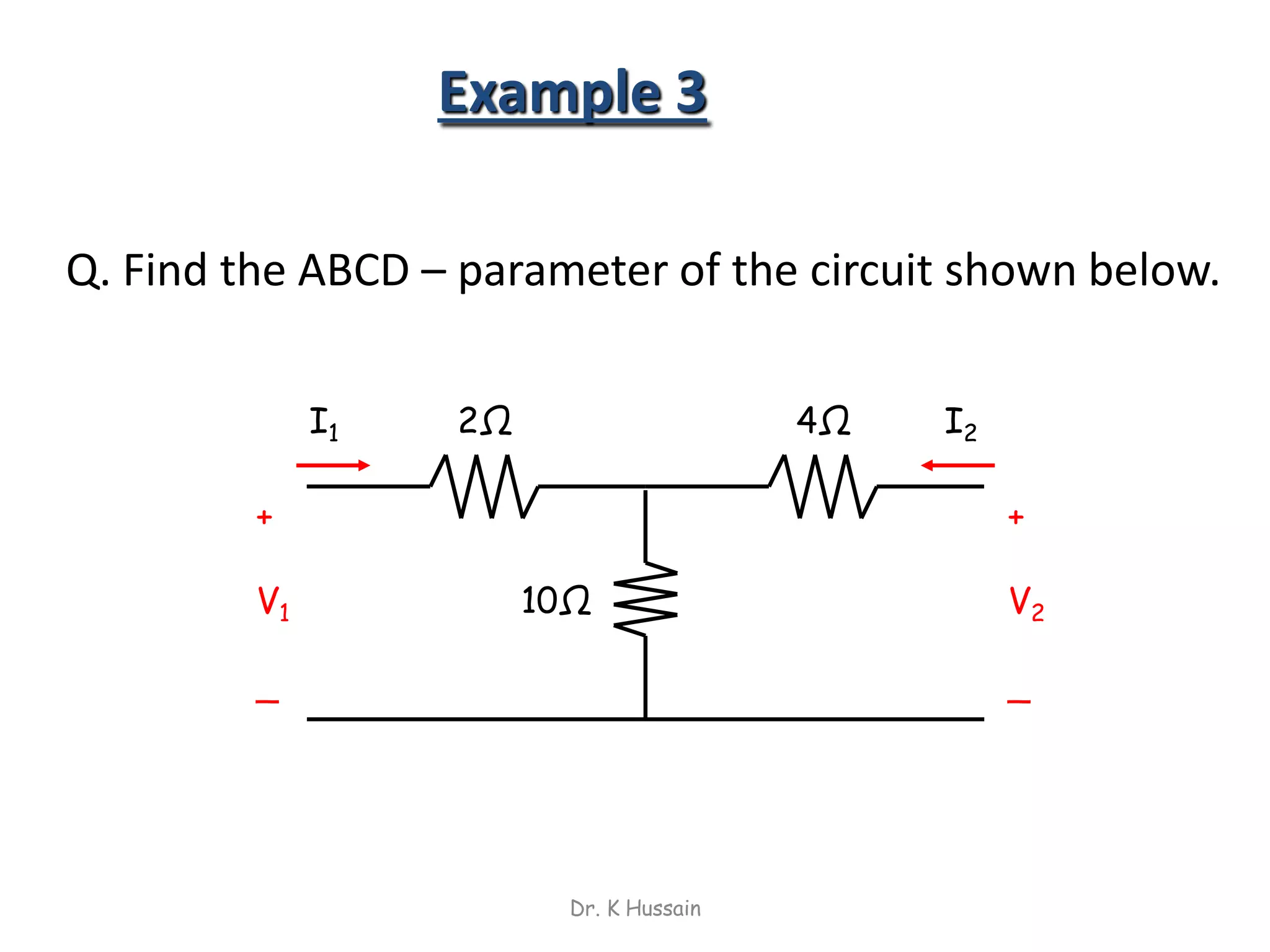
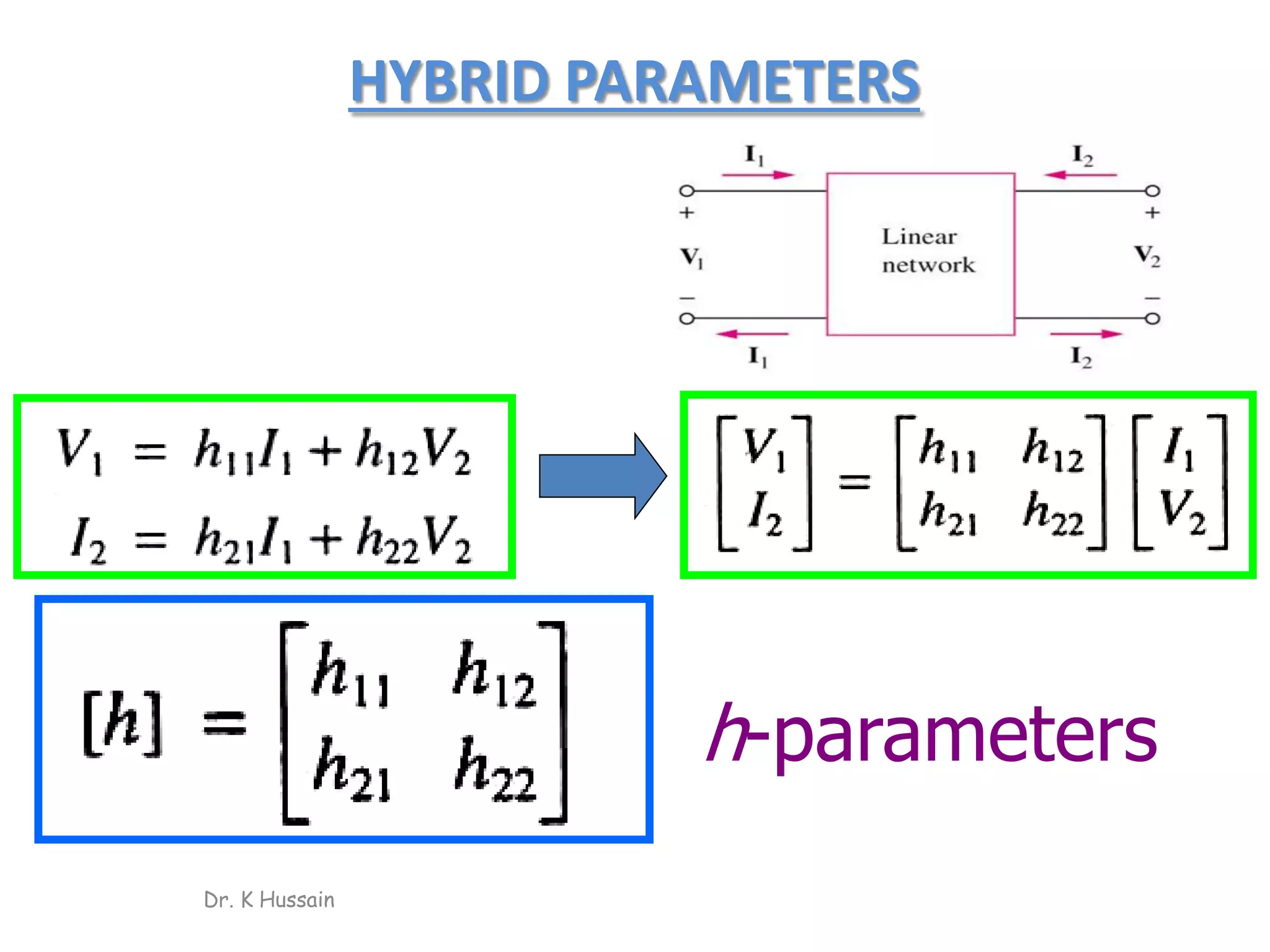
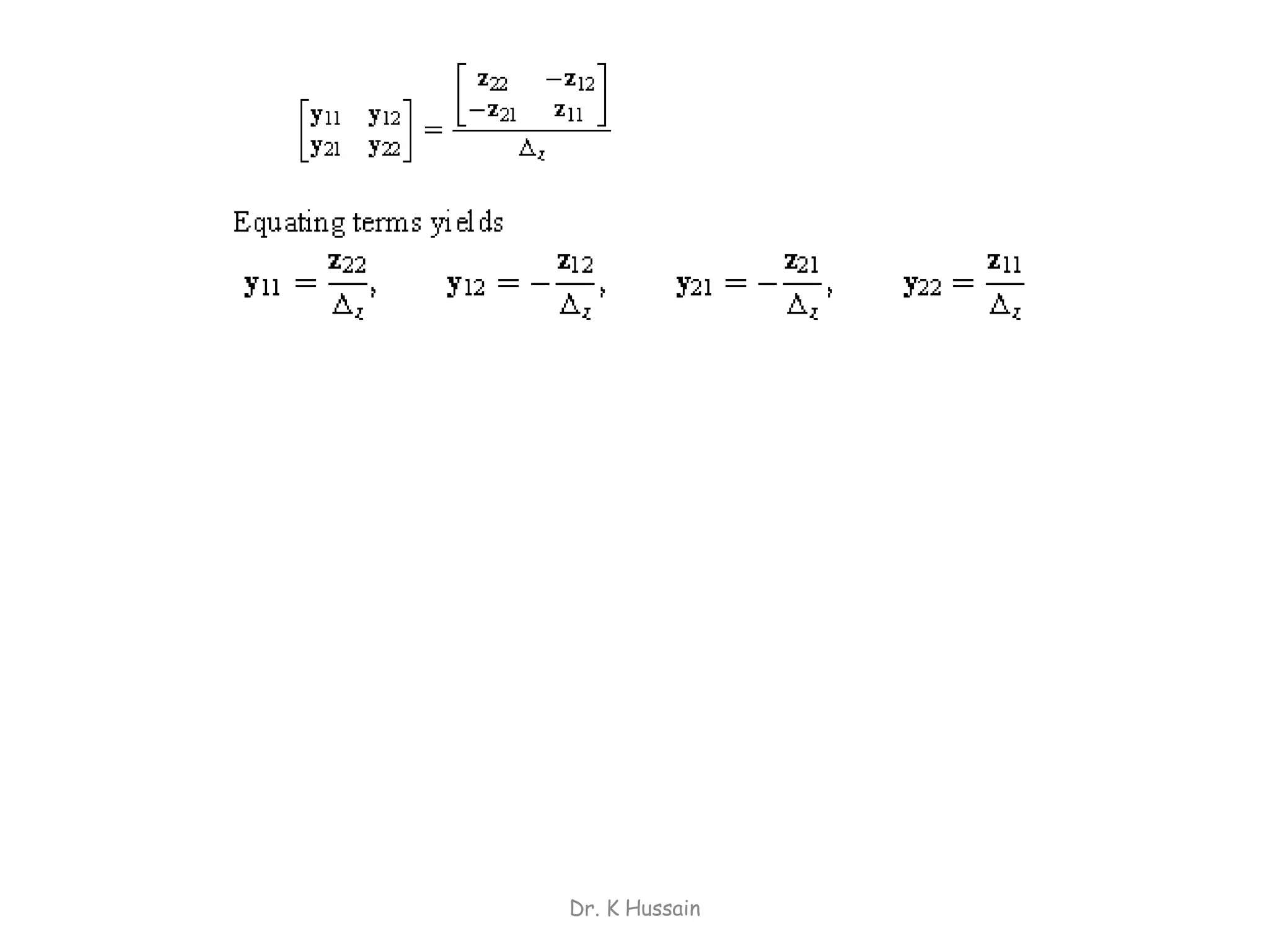
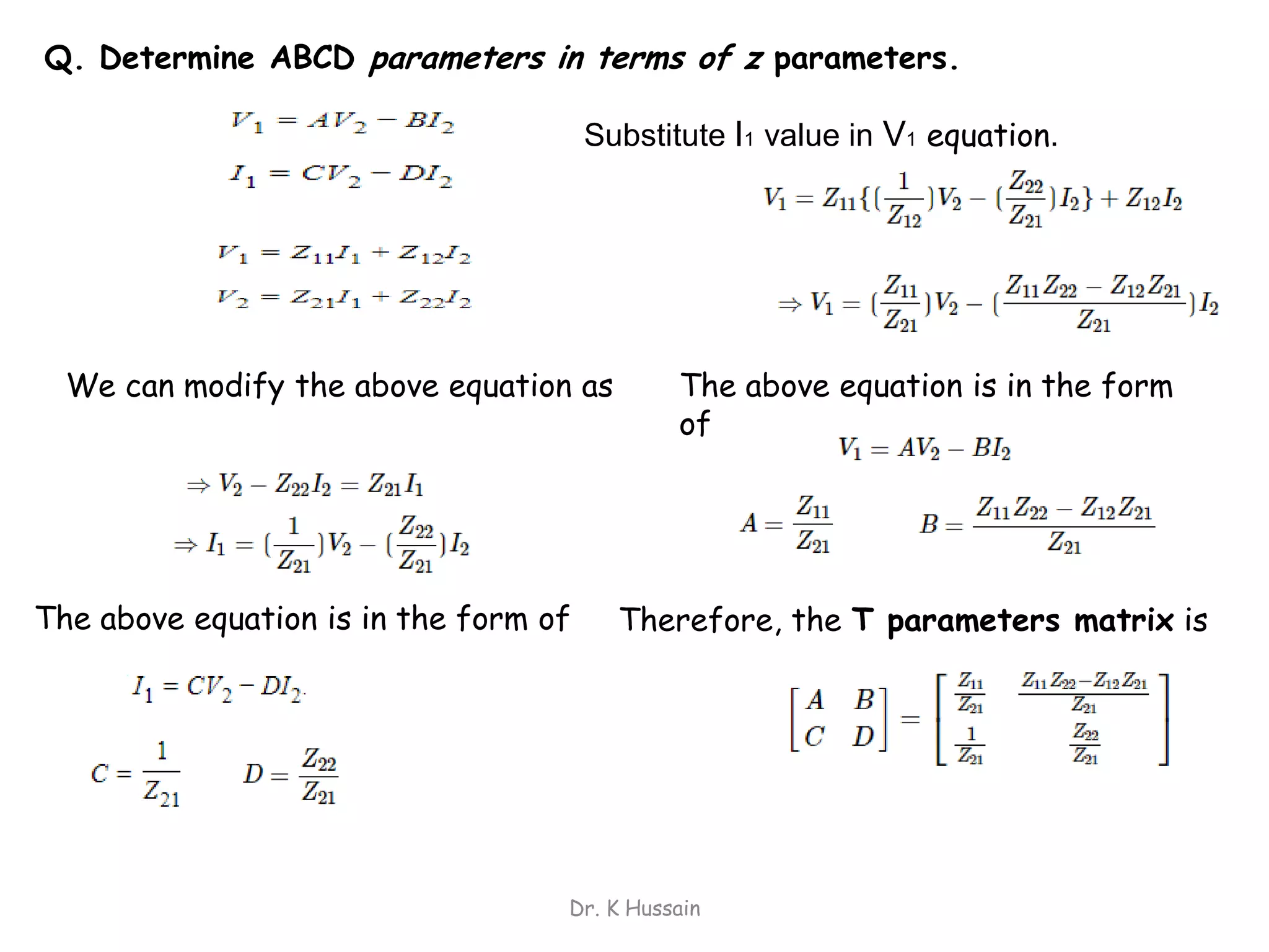
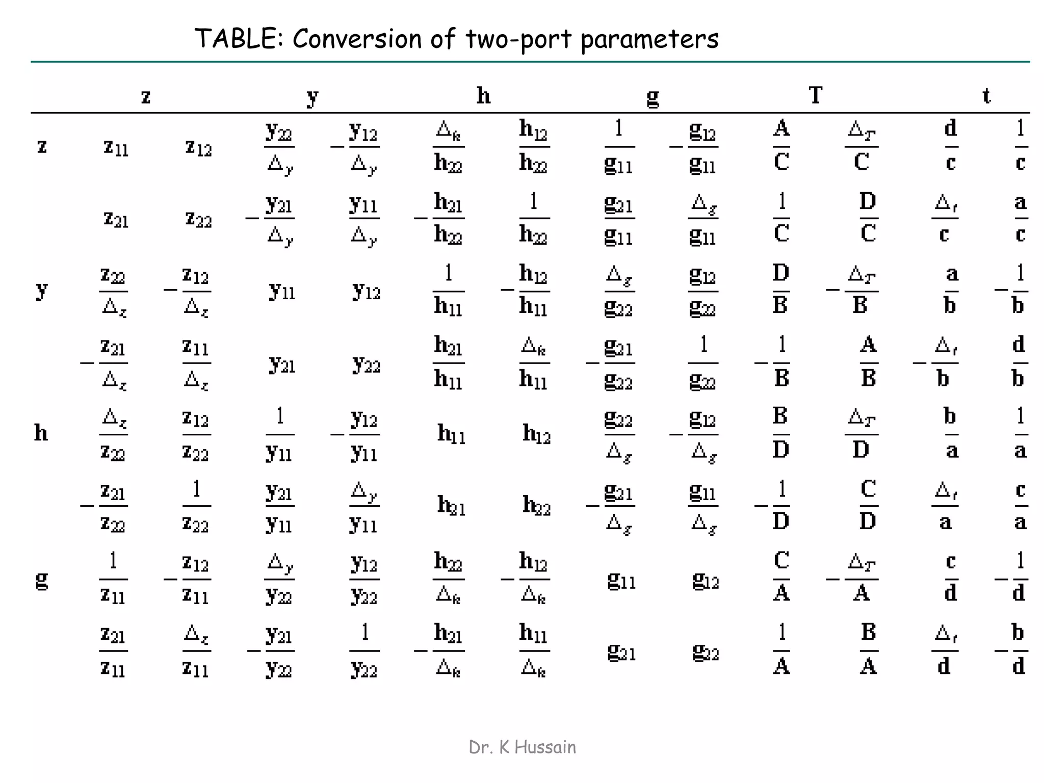
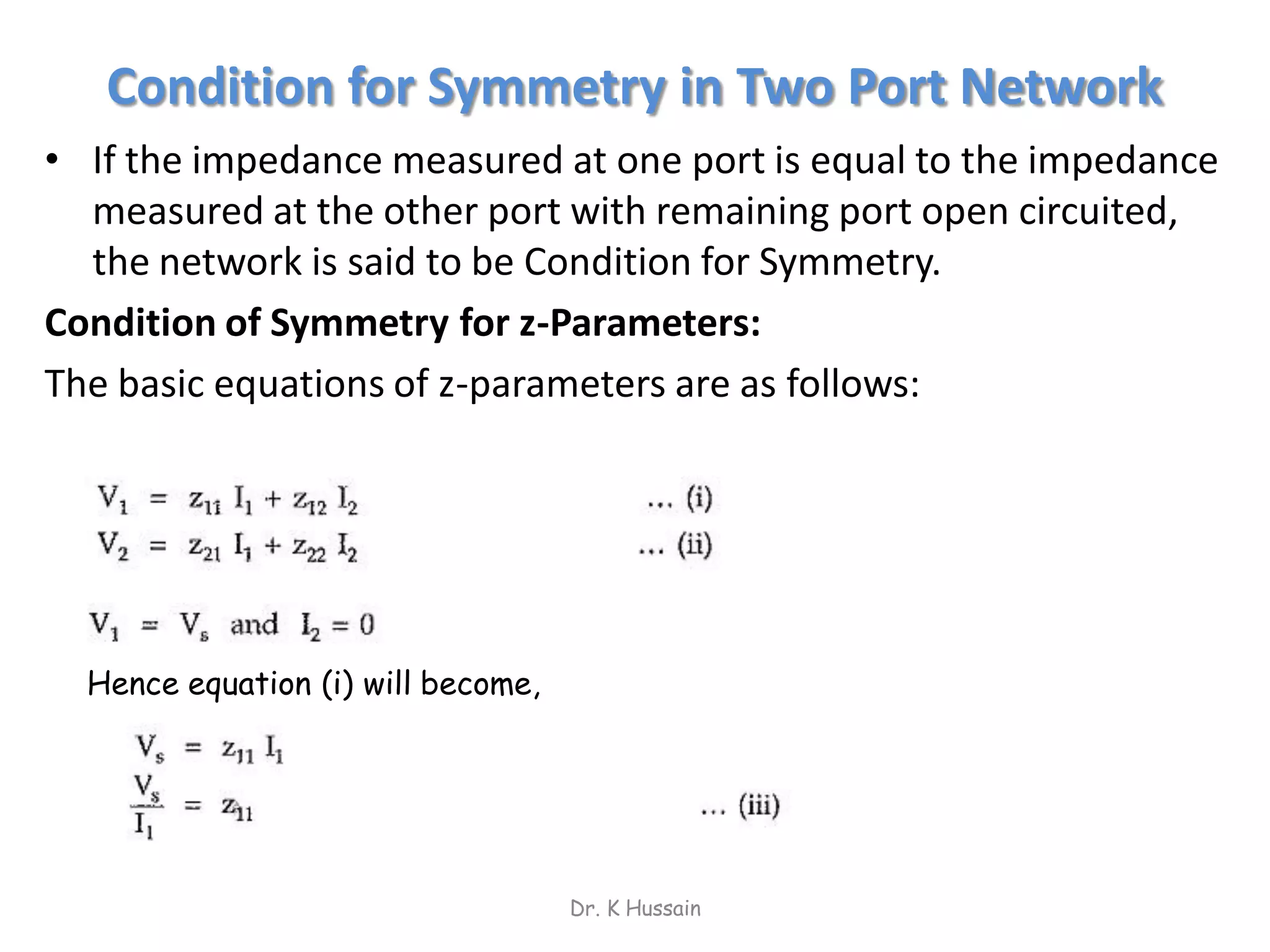
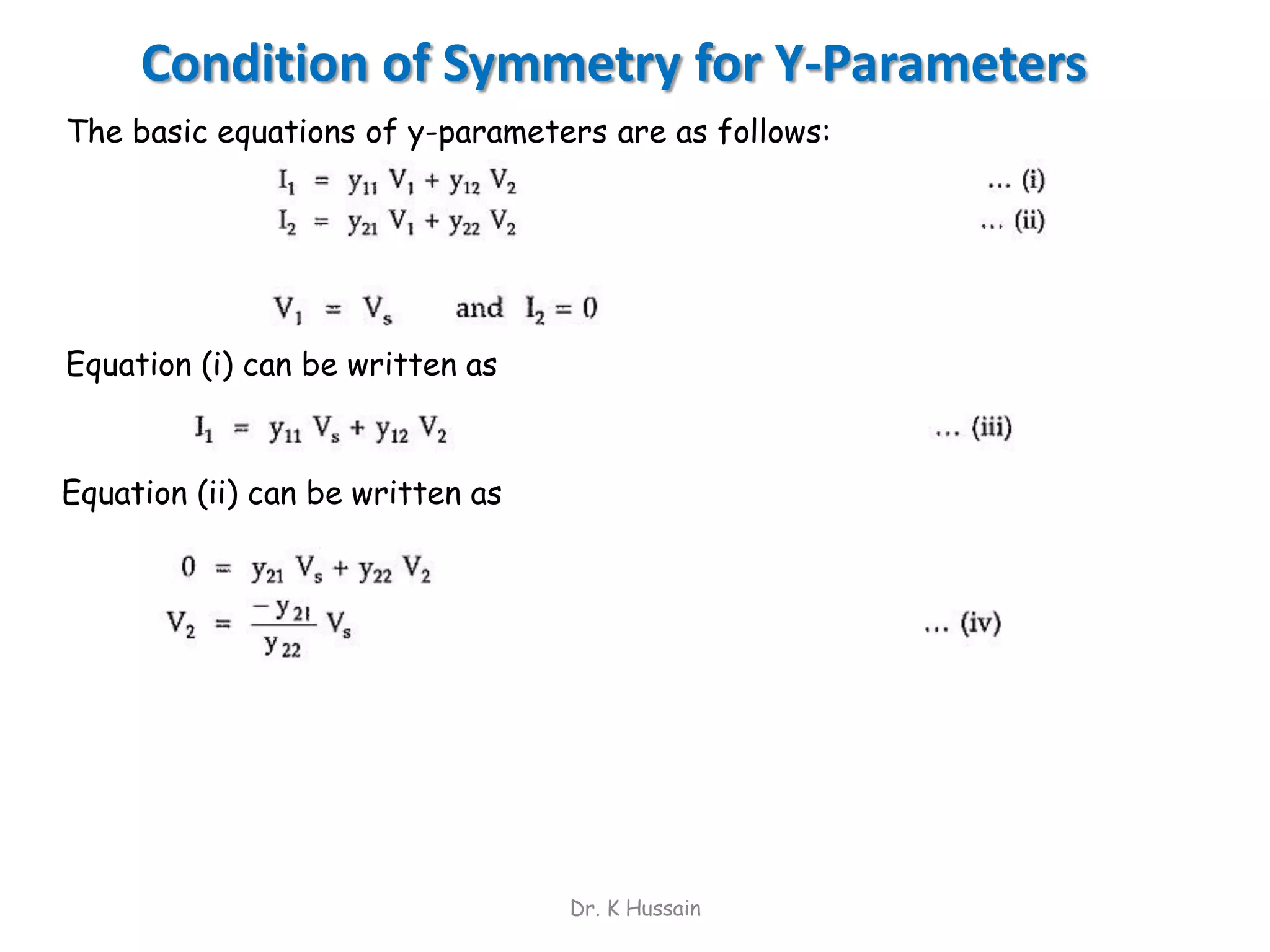
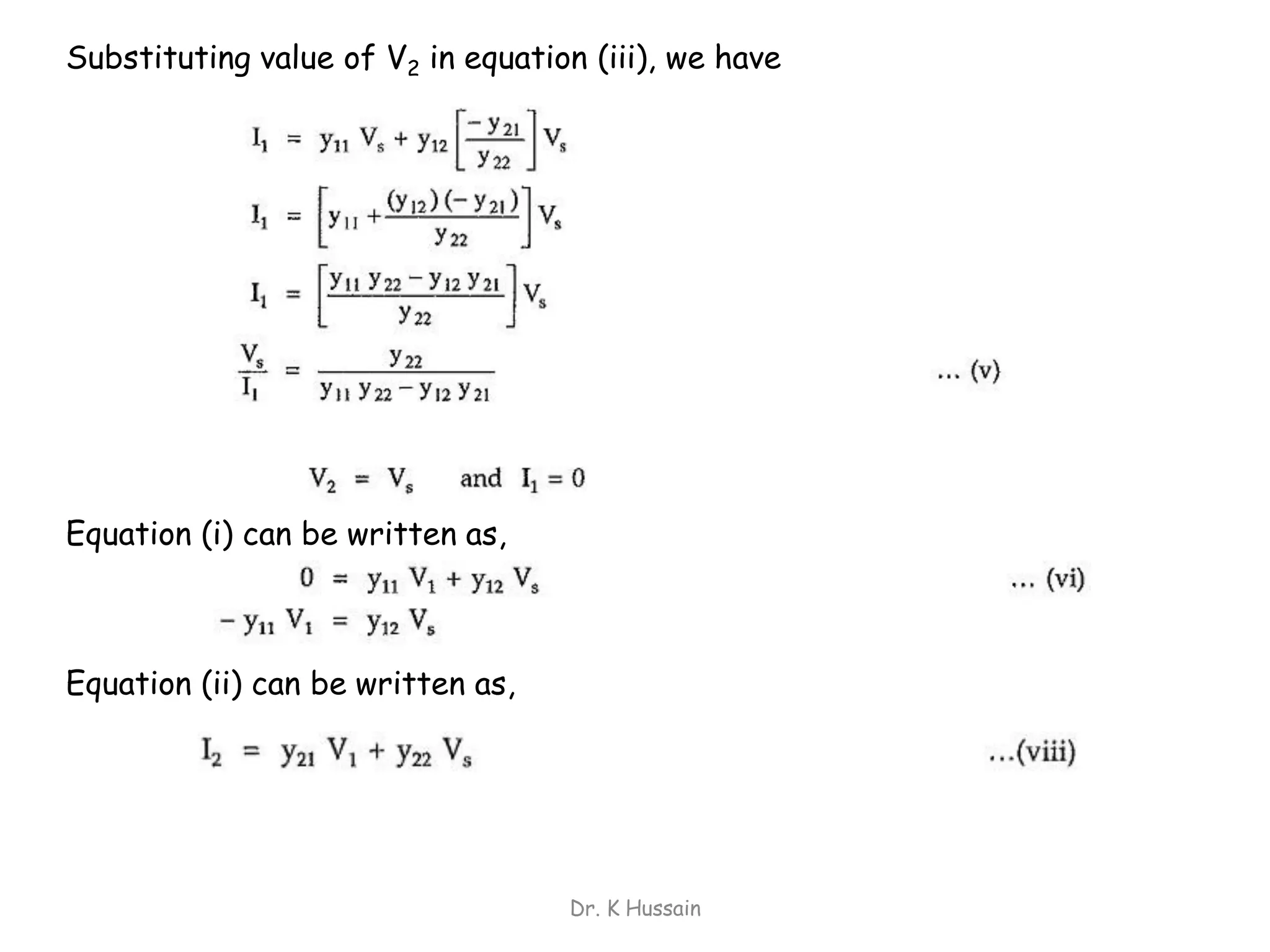
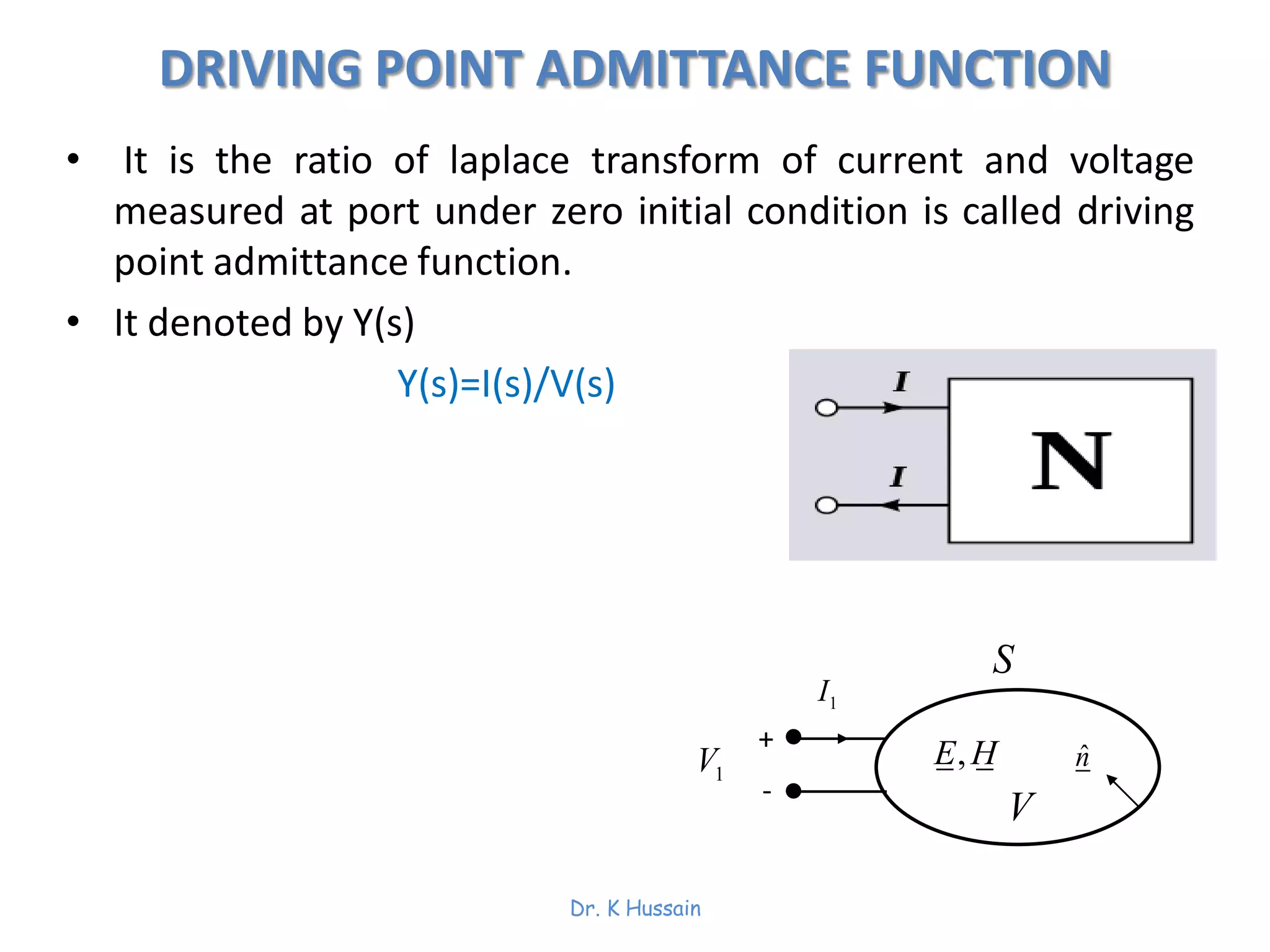
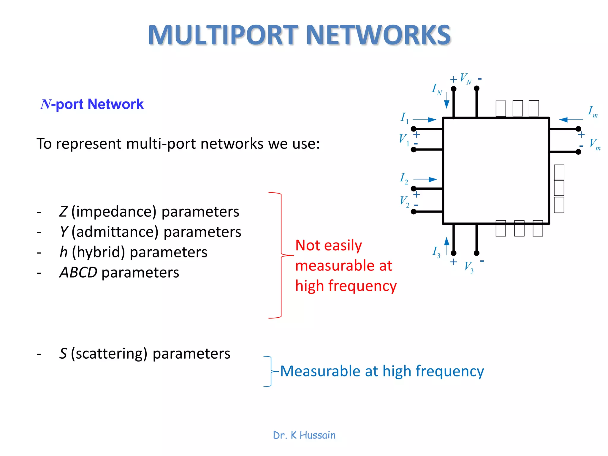
Chapter 5 discusses two-port networks, including definitions, parameters (z, y, abcd), and their significance in electrical engineering. It explains various classifications of parameters, examples of parameter calculations, and how these networks can be interconnected. The text also covers conditions for symmetry and reciprocity in two-port networks.

1. CHAPTER-5
TWO PORT NETWORKS
by
Dr. K Hussain
Associate Professor & Head,
Dept. of EE, SITCOE

2. OBJECTIVES
• To understand about two – port networks and its
functions.
• To understand the different between z-
parameter, y-parameter, ABCD- parameter and
terminated two port networks.
• To investigate and analysis the behavior of two –
port networks.
Dr. K Hussain

3. TWO – PORT NETWORKS
• A pair of terminals through which a current may enter or leave a
network is known as a port.
• Two terminal devices or elements (such as resistors, capacitors,
and inductors) results in one – port network.
• Most of the circuits we have dealt with so far are two – terminal
or one –port circuits. (Fig. a)
• A two – port network is an electrical network with two separate
ports for input and output.
Dr. K Hussain

4. Dr. K Hussain
One port or two
terminal circuit
Two port or four
terminal circuit
• It is an electrical
network with two
separate ports for
input and output.
• No independent
sources.
It has two terminal pairs acting as access points. The current entering
one terminal of a pair leaves the other terminal in the pair. (Fig. b)

5. Z – PARAMETER
• Z – parameter also called as impedance parameter and the unit is
ohm (Ω)
• The “black box” is replace with Z-parameter is as shown below.
Dr. K Hussain
+
V1
-
I1
I2
+
V2
-
Z11
Z21
Z12
Z22
2221212
2121111
IzIzV
IzIzV


  























2
1
2
1
2221
1211
2
1
I
I
z
I
I
zz
zz
V
V
where the z terms are called the impedance parameters, or
simply z parameters, and have units of ohms.

6. Dr. K Hussain
z11 = Open-circuit input impedance
z21 = Open-circuit transfer
impedance from port 1 to port 2
z12 = Open-circuit transfer
impedance from port 2 to port 1
z22 = Open-circuit output
impedance
0I1
2
21
0I1
1
11
22
I
V
zand
I
V
z


0I2
2
22
0I2
1
12
11
I
V
zand
I
V
z



7. Example 1
Q. Find the Z – parameter of the circuit below.
40Ω
240Ω
120Ω
+
V1
_
+
V2
_
I1
I2
Dr. K Hussain

8. Solution
40Ω
240Ω
120Ω
+
V
1
_
+
V2
_
I1
Ia
Ib
When I2 = 0(open circuit port 2). Redraw the circuit.




84
(2)(1)sub
)2......(
400
280
)1.......(120
1
1
11
1
1
I
V
Z
II
IV
b
b




72
(3)(4)sub
)4.......(
400
120
.......(3)240
1
2
21
1
2
I
V
Z
II
IV
a
a
Dr. K Hussain

9. 40Ω
240Ω
120Ω
+
V1
_
+
V2
_
Iy I2
Ix
When I1 = 0 (open circuit port 1). Redraw the circuit.




96Z
(2)(1)sub
)2.......(
400
160
)1.......(240
2
2
22
2
2
I
V
II
IV
x
x




72
(3)(4)sub
)4.......(
400
240
)3.......(120
2
1
12
2
1
I
V
Z
II
IV
y
y
  






9672
7284
ZIn matrix form:
Dr. K Hussain

10. Y - PARAMETER
• Y – parameter also called admittance parameter and the unit is
Siemens (S).
• The “black box” that we want to replace with the Y-parameter is
shown below.
Dr. K Hussain
+
V1
-
I1
I2
+
V2
-
Y11
Y21
Y12
Y22
2221212
2121111
VyVyI
VyVyI


  























2
1
2
1
2221
1211
2
1
V
V
y
V
V
yy
yy
I
I
where the y terms are called the admittance parameters, or
simply y parameters, and they have units of Siemens.

11. Dr. K Hussain
0V2
2
22
0V2
1
12
11
V
I
yand
V
I
y


y11 = Short-circuit input
admittance
y21 = Short-circuit transfer
admittance from port 1 to port 2
y12 = Short-circuit transfer
admittance from port 2 to port 1
y22 = Short-circuit output
admittance
0V1
2
21
0V1
1
11
22
V
I
yand
V
I
y



12. Example 2
Q. Find the Y – parameter of the circuit shown below.
5Ω
15Ω20Ω
+
V1
_
+
V2
_
I1
I2
Dr. K Hussain

13. Solution
i) V2 = 0
5Ω
20Ω
+
V1
_
I1
I2
Ia S
V
I
Y
II
IV
a
a
4
1
(2)(1)sub
)2.......(
25
5
)1.......(20
1
1
11
1
1




S
V
I
Y
IV
5
1
5
1
2
21
21


Dr. K Hussain

14. ii) V1 = 0
In matrix form;
5Ω
15Ω
+
V2
_
I1
I2
Ix
S
V
I
Y
II
IV
x
x
15
4
(4)(3)sub
)4.......(
20
5
)3.......(15
2
2
22
2
2




S
V
I
Y
IV
5
1
5
2
1
12
12


  SY













15
4
5
1
5
1
4
1
Dr. K Hussain

15. T (ABCD) PARAMETER
• T – parameter or also ABCD – parameter is a another set of
parameters relates the variables at the input port to those at
the output port.
• T – parameter also called transmission parameters because
this parameter are useful in the analysis of transmission lines
because they express sending – end variables (V1 and I1) in
terms of the receiving – end variables (V2 and -I2).
• The “black box” that we want to replace with T – parameter
is as shown below.
Dr. K Hussain
+
V1
-
I1
I2
+
V2
-
A11
C21
B12
D22

16. Dr. K Hussain
221
221
DICVI
BIAVV


  
























2
2
2
2
1
1
I
V
T
I
V
DC
BA
I
V
where the T terms are called the transmission parameters,
or simply T or ABCD parameters, and each parameter has
different units.
0I2
1
0I2
1
2
2
V
I
C
V
V
A




0V2
1
0V2
1
2
2
I
I
D
I
V
B




A=open-circuit
voltage ratio
C= open-circuit
transfer admittance
(S)
B= negative short-
circuit transfer
impedance ()
D=negative short-
circuit current ratio

17. Example 3
Q. Find the ABCD – parameter of the circuit shown below.
2Ω
10Ω
+
V2
_
I1 I2
+
V1
_
4Ω
Dr. K Hussain

18. Solution
i) I2 = 0,
2Ω
10Ω
+
V2
_
I1
+
V1
_
2.1
5
6
10
2
2
1.0
10
2
1
22
2
1
211
2
1
12











V
V
A
VV
V
V
VIV
S
V
I
C
IV
Dr. K Hussain

19. ii) V2 = 0,
 












8.6
10
10
14
12
1012
102
4.1
14
10
2
1
221
211
2111
2
1
12
I
V
B
IIV
IIV
IIIV
I
I
D
II
2Ω
10Ω
I1 I2
+
V1
_
4Ω
I1 + I2
  




 

4.11.0
8.62.1
S
T
In matrix form;
Dr. K Hussain

20. HYBRID PARAMETERS
Dr. K Hussain
h-parameters

21. Dr. K Hussain
1. Input impedance with output short-circuited
2
1
11
1 0V
V
h
I 
 
2. Reverse voltage gain with input open-circuited
1
1
12
2 0I
V
h
V 


22. Dr. K Hussain
3. Forward current gain with output short-circuited
2
2
21
1 0V
I
h
I 

4. Output admittance with input open-circuited
1
2
22
2 0
S
V
I
h
V 


23. • Note that the four h-parameters have mixed
dimensions.
• This is the reason why these parameters are called
hybrid parameters.
• Using h-parameter equivalent circuit for a transistor
proves beneficial in two ways.
• Firstly, the measurement of these parameters for a
transistor is quite easy.
• Secondly, the analysis of the transistor amplifier
becomes much simpler.
Dr. K Hussain

24. Dr. K Hussain
Example: Find the hybrid parameters for the two-port network of Fig.
To find h11 and h21, we short-circuit the
output port and connect a current
source I1 to the input port as shown in
Fig.(a). From Fig.(a),
Also, from Fig. (a) we obtain, by current division,
Solution:

25. Dr. K Hussain
To obtain h12 and h22, we open-circuit the input port and connect a
voltage source V2 to the output port as in Fig. (b). By voltage division,

26. RELATIONSHIPS BETWEEN PARAMETERS
• Since the six sets of parameters relate the same input and output terminal
variables of the same two-port network, they should be interrelated.
Dr. K Hussain
Q. Determine the y-Parameters in terms of z-Parameters.

27. Dr. K Hussain

28. Dr. K Hussain
Q. Determine ABCD parameters in terms of z parameters.
The above equation is in the form
of
We can modify the above equation as
The above equation is in the form of
Substitute I1 value in V1 equation.
Therefore, the T parameters matrix is

29. Dr. K Hussain
Q. Determine the h parameters in terms of z parameters.
Making I2 the subject of Eq.
Substituting this into Eq.
Putting Eqs. (V1) and (I2) in matrix form
Comparing this with Eq., we obtain

30. Dr. K Hussain
TABLE: Conversion of two-port parameters

31. Dr. K Hussain

32. Dr. K Hussain
Exercise1: Determine z, y & ABCD parameters from h-parameters.
Exercise2: Determine z, ABCD & h parameters from y-parameters.
Exercise3: Determine z, y & h parameters from ABCD-parameters.
Exercise 4: Find out condition of symmetry and reciprocity?

33. Conditions for Symmetry & Reciprocity
Dr. K Hussain

34. Condition for Symmetry in Two Port Network
• If the impedance measured at one port is equal to the impedance
measured at the other port with remaining port open circuited,
the network is said to be Condition for Symmetry.
Condition of Symmetry for z-Parameters:
The basic equations of z-parameters are as follows:
Dr. K Hussain
Hence equation (i) will become,

35. Equation (ii) can be written as,
Dr. K Hussain
For symmetrical networks, both the port impedances must be equal i.e.,
Condition of Symmetry for z-Parameters ..Contd..

36. Dr. K Hussain
Condition of Symmetry for Y-Parameters
The basic equations of y-parameters are as follows:
Equation (i) can be written as
Equation (ii) can be written as

37. Dr. K Hussain
Equation (ii) can be written as,
Substituting value of V2 in equation (iii), we have
Equation (i) can be written as,

38. Dr. K Hussain
For symmetrical networks, both the port impedances must be equal i.e.,
Substituting value of V1 in equation (viii) from equation (vii), we have

39. Dr. K Hussain
Condition of Symmetry for Transmission Parameters
The basic equations for the transmission parameters are as following
Equation (ii) can be written as,
Equation (i) can be written as,
Case (i)

40. Dr. K Hussain
For the symmetrical network, both the port impedances must be equal.
Equation (ii) can be written as,
Equation (i) can be written as,
Case (ii)

41. Dr. K Hussain
Conditions of Symmetry for h-Parameters
The basic equations of h-parameters are as follows,
Equation (ii) can be written as
Equation (i) can be written as,
Case (i):

42. Dr. K Hussain
Substituting value of V2 in equation (iii), we have
Equation (i) can be written as
Equation (ii) can be written as
For symmetrical networks, both the port impedances must be equal i.e.,
Case (ii):

43. Dr. K Hussain
Additional Topics

44. Dr. K Hussain
INTERCONNECTION OF NETWORKS
A large, complex network may be divided into subnetworks for the
purposes of analysis and design. The subnetworks are modeled as
two-port networks, interconnected to form the original network.
The two-port networks may therefore be regarded as building
blocks that can be interconnected to form a complex network. The
interconnection can be in series, in parallel, or in cascade. Although
the interconnected network can be described by any of the six
parameter sets, a certain set of parameters may have a definite
advantage.
For ex:
when the networks are in series, their individual z parameters add up
to give the z parameters of the larger network.
When they are in parallel, their individual y parameters add up to
give the y parameters the larger network.
When they are cascaded, their individual transmission parameters
can be multiplied together to get the transmission parameters of
the larger network.

45. Dr. K Hussain
Consider the series connection of two-port networks shown in Fig. 1. The
networks are regarded as being in series because their input currents are the
same and their voltages add.
For network Na,
For network Nb,
SERIES CONNECTION OF TWO-PORT NETWORKS
It is showing that the z parameters for the overall network are the sum of the
z parameters for the individual networks.
Fig. 1
In addition, each network has a common reference, and when the circuits are
placed in series, the common reference points of each circuit are connected
together.

46. Dr. K Hussain
Two two-port networks are in parallel when their port voltages are equal and
the port currents of the larger network are the sums of the individual port
currents. In addition, each circuit must have a common reference and when
the networks are connected together, they must all have their common
references tied together. The parallel connection of two two-port networks is
shown in Fig. 2.
For the two networks
Thus, the y parameters for the overall network are
It is showing that the y parameters of the overall network are the sum of
the y parameters of the individual networks.
PARALLEL CONNECTION OF TWO-PORT NETWORKS
Fig. 2

47. Dr. K Hussain
The connection of two two-port networks in
cascade is shown in Fig 3.
For the two networks,
Substituting these into Eqs.
Thus, the transmission parameters for the overall network are the product
of the transmission parameters for the individual transmission parameters:
It is this property that makes the transmission parameters so useful.
Keep in mind that the multiplication of the matrices must be in the order in
which the networks Na and Nb are cascaded.
CASCADE CONNECTION OF TWO-PORT NETWORKS
Fig. 3

48. ONE PORT NETWORK
• A port is combination of two terminals on the same side of
network. Thus a terminal pair is nothing but a port as shown in
fig .
• A network having only one terminal pair or port is called one
port network.
• One port network can be represented as below.
R
1I
1V
+
-
+
-

1I
1V
Dr. K Hussain

49. NETWORK FUNCTION FOR ONE PORT NETWORK
• Voltage and current for the one port linear network as shown
in fig.
• As there is one port , voltage and current measured at same
port. thus for one port network only driving function can be
defined as below.
DRIVING POINT IMPEDANCE FUNCTION:
• The ratio of laplace transform of voltage and current measured
at port under zero initial condition is called driving point
impedance function
• It is denoted by Z(s)
Z(s)=V(s)/I(s)
Dr. K Hussain

50. DRIVING POINT ADMITTANCE FUNCTION
• It is the ratio of laplace transform of current and voltage
measured at port under zero initial condition is called driving
point admittance function.
• It denoted by Y(s)
Y(s)=I(s)/V(s)
,E H ˆn
S
V
1V
1I
+
-
Dr. K Hussain

51. N-port Network
To represent multi-port networks we use:
- Z (impedance) parameters
- Y (admittance) parameters
- h (hybrid) parameters
- ABCD parameters
- S (scattering) parameters
Not easily
measurable at
high frequency
Measurable at high frequency
MULTIPORT NETWORKS
 




+
+
+
+
+
1I
2I
3I
mI
NI
1V
2V
3V
mV
NV
-
-
-
-
-
Dr. K Hussain

52. NETWORK FUNCTIONS FOR TWO-PORT NETWORK
• Consider a two port network with voltages and currents at ports
1-1’ and 2-2’ as V1(t), I1(t) and V2(t), I2(t) respectively as shown in
figure.
Dr. K Hussain
1
1’
2
2’

53. NETWORK FUNCTIONS FOR TWO-PORT NETWORKS
1. Driving Point Functions:
• Driving point impedance functions
• Driving point admittance functions
2. Transfer Functions:
• Voltage transfer functions
• Current transfer functions
• Transfer impedance functions
• Transfer admittance functions
Dr. K Hussain

54. DRIVING POINT FUNCTIONS
Driving Point Impedance Functions:
• The ratio of Laplace transform of voltage and current at port 1-1’
or 2-2’ is defined as driving point impedance function.
Two types of driving point impedance functions:
• At port 1-1’ denoted as Z11(s)
Z11(s)= V1(s)/I1(s)
• At port 2-2’ denoted as Z22(s)
Z22(s)= V2(s)/I2(s)
Dr. K Hussain
1
1’
2
2’

55. DRIVING POINT FUNCTIONS
Driving Point Admittance Functions:
• The ratio of Laplace transform of current and voltage at port 1-1’
or 2-2’ is defined as driving point admittance function.
Two types of driving point admittance functions:
• At port 1-1’ denoted as Y11(s)
Y11(s)=I1(s)/V1(s)
• At port 2-2’ denoted as Y11(s)
Y22(s)=I2(s)/V2(s)
Dr. K Hussain
1
1’
2
2’

56. TRANSFER FUNCTIONS
Voltage Transfer Function:
• It is defined as the ratio of Laplace transform of voltage at one
port and voltage at another port.
• It is denoted as G(s).
• G12(s) =V1(s)/V2(s)
and G21(s) =V2(s)/V1(s)
Current Transfer Function:
• It is defined as the ratio of Laplace transform of current at one
port and current at another port.
• It is denoted as (s).
• 12(s) = I1(s)/I2(s) and 21(s) =I2(s)/I1(s)
Dr. K Hussain
1
1’
2
2’

57. TRANSFER FUNCTIONS
Transfer Impedance Function:
• It is defined as the ratio of Laplace transform of voltage at one
port and current at another port.
Z12(s)=V1(s)/I2(s) and Z21(s)=V2(s)/I1(s)
Transfer Admittance Function:
• It is defined as the ratio of Laplace transform of current at one
port and voltage at another port.
Y12(s) =I1(s)/V2(s) and Y21(s) =I2(s)/V1(s)
Dr. K Hussain

58. Dr. K Hussain
CONCEPT OF POLES AND ZEROS
The transfer function provides a basis for determining important system
response characteristics without solving the complete differential equation.
As defined, the transfer function is a rational function in the complex
variable s = σ + jω, that is
It is often convenient to factor the polynomials in the numerator and
denominator, and to write the transfer function in terms of those factors:
where the numerator and denominator polynomials, N(s) and D(s), have real
coefficients defined by the system’s differential equation and K = bm/an.
As written in Eq. (2) the zi’s are the roots of the equation N(s) = 0, and are
defined to be the system zeros, and the pi’s are the roots of the equation
D(s) = 0, and are defined to be the system poles.

59. Dr. K Hussain
Together with the gain constant K they completely characterize the
differential equation, and provide a complete description of the system.
Example: A system has a pair of complex conjugate poles p1, p2 = −1j2, a single
real zero z1 = −4, and a gain factor K = 3. Find the differential equation
representing the system.
Solution: The transfer function is
and the differential equation is
Figure 1: The pole-zero plot for a typical third-order system with one real pole
and a complex conjugate pole pair, and a single real zero.
The poles and zeros are properties of the transfer function, and therefore
of the differential equation describing the input-output system dynamics.

60. Dr. K Hussain
Example:
A linear system is described by the differential equation
Find the system poles and zeros.
which may be written in factored form
The system therefore has a single real zero at s = −1/2, and a pair of
real poles at s = −3 and s = −2.
Solution: From the differential equation the transfer function is

61. Dr. K Hussain
Two more important applications:
Network Stability and
Network Synthesis.
APPLICATIONS
So far we have considered three applications of Laplace’s transform:
circuit analysis in general, obtaining transfer functions, and solving
linear Integro-differential equations.
The Laplace transform also finds application in other areas in circuit
analysis, signal processing, and control systems.

62. Dr. K Hussain
Network Synthesis
Network synthesis may be regarded as the process of obtaining an appropriate
network to represent a given transfer function.
Network synthesis is easier in the s domain than in the time domain
In network analysis, we find the transfer function of a given network.
In network synthesis, we reverse the approach: given a transfer function, we
are required to find a suitable network.
Network synthesis is finding a network that represents a given transfer
function.
Keep in mind that in synthesis, there may be many different answers—or
possibly no answers—because there are many circuits that can be used to
represent the same transfer function; in network analysis, there is only one
answer.
Network synthesis is an exciting field of prime engineering importance.
Being able to look at a transfer function and come up with the type of circuit it
represents is a great asset to a circuit designer. Although network synthesis
constitutes a whole course by itself and requires some experience, the
following examples are meant to whet your appetite.

63. Dr. K Hussain
Example: Given the transfer function
Realize the function using the circuit in Fig.(a).
(a) Select R = 5 , and find L and C. (b) Select R = 1 , and find L and C.
The s-domain equivalent of the circuit in Fig. (a) is shown in Fig. (b).
The parallel combination of R and C gives
Using the voltage division principle,
Comparing this with the given transfer function H(s) reveals that
There are several values of R, L, and C that satisfy these requirements.
This is the reason for specifying one element value so that others can be
determined.
Solution:

64. Dr. K Hussain
(a) If we select R = 5 , then
(b) If we select R = 1 , then