Download as PDF, PPTX
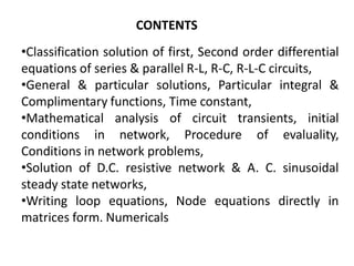
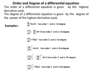
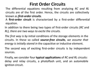
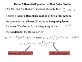
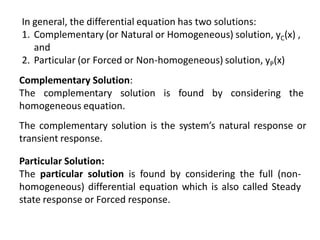
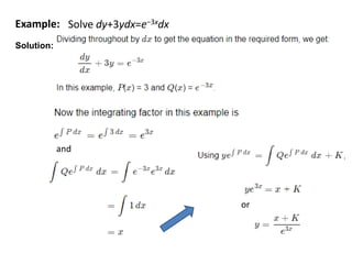
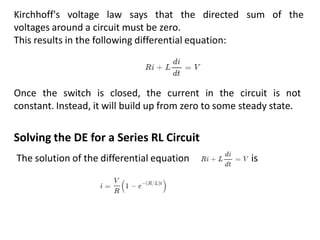
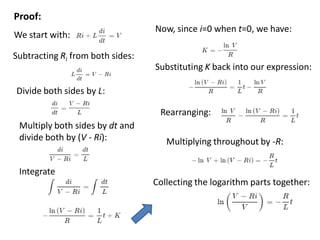
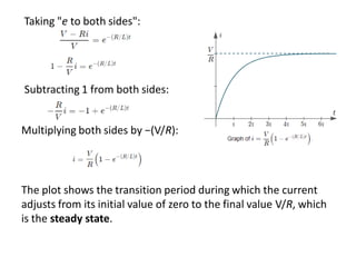
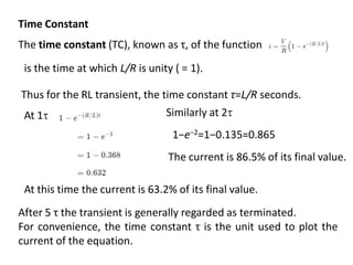
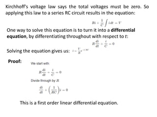
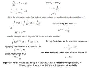
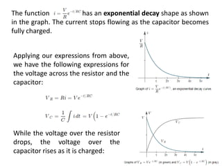
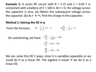
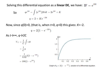
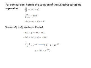
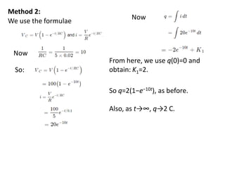
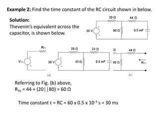
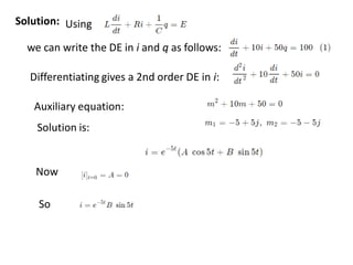
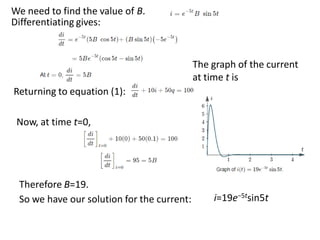
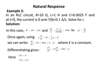
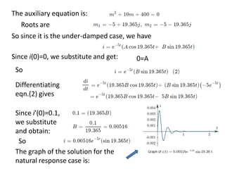


Chapter 3 explores the solutions of network equations for R-L, R-C, and R-L-C circuits, focusing on first and second order differential equations. It discusses the complementary and particular solutions, time constants, and responses of circuits under transient and steady-state conditions, including applications of RC and RL circuits. Additionally, it covers the formation of differential equations, solving techniques, and examples involving source-free circuits and the use of Kirchhoff's laws.