1. The document introduces complex numbers and some basic results regarding complex numbers such as the complex conjugate and modulus of a complex number. 2. It then discusses functions of a complex variable, defining a complex function and its Cartesian and polar forms. It also covers continuity, derivatives, and analytic functions of a complex variable. 3. The Cauchy-Riemann equations are derived and provide a necessary condition for a function to be analytic (differentiable everywhere in a neighborhood). Two examples are provided to illustrate the Cauchy-Riemann equations and analytic functions.

1. Unit_III
Complex Numbers:
In the system of real numbers R we can solve all quadratic equations of the
form
0,0x2
≠=++ acbxa , and the discriminant 042
≥− acb . When the discriminant
042
<− acb , the solution of this quadratic equation do not belong to the
system of .
In fact , a simple quadratic equation of the form 012
=+x , does possesses
solution in real. This difficulty was overcame by introducing the imaginary
part unit i, where 12
−=i .
Thus the set of complex numbers defined as . }{ 1,:)( −=∈+= iandRyxiyxC .
Some Basic Results:
1. If z = x +iy is a complex number, then the complex number iyxz −= is
called the complex conjugate of z , and 22
))((zz yxiyxiyx +=−+=
2.If z= x+iy is a complex number , then the modulus of z, denoted by
22
yz += x
3. A complex number z = x + iy is represented by a point p(x ,y) in the
Cartesian plane with abscissa x and ordinate y. Then the x-axis is called real
axis and the y-axis is called the imaginary axis.The point p(x, y) is referred
to as the point z.
Let OP= r and .θ=∠XOP Then θθ rsiny,cosrx ==
Every Complex number can z = x +iy be expressed in the form as given
below
)isinr(cosz θθ += polar form
θi
rez = exponential form
We observe that
22xr y+= the modulus of z and it represents the
distance of the point z from the origin. Also
.argtanθ 1-
zofumentthecalledisanglethe
x
y
θ





=
4. Let 000z iyx += then )()(z-z 000 yyixx −+−=
( ) ( )2
0
2
0 yyxx −+−= .
Now 0z-z may be represented as

2. )sin(cosz-z 0 θθ iR += and Rzz =− 0 serves as the complex equation
of the circle C with ( )00 , yx and radius R. In particular 1z = represents the
circle with center at the origin and radius equal to 1.
Functions of a complex variable:
Let C be a set complex numbers. If to each complex number z in C there
corresponds a unique complex number w ., then w is called a complex
function of z defined on C, and we write w = f(z). Hence ,w has a real part ,
say u and an imaginary part , say v. Then , w has the representation
W= f(z) = u(x,y) + i v(x,y) (Cartesian form)
W = u(r,θ) + i v(r,θ) (polar form)
Continuity :
A complex valued function f(z) is said to be continuous at a point 0z if f(z)
is defined at 0z and 0zz
zf(z)lim0
=→
.
Note:
1. If a complex valued function f(z) is differentiable at a point 0z , then
it is continuous at 0z .
2. The converse of the above result is not always true. The continuity of
a complex function need not imply its differentiability.
Derivative of a complex function:
The derivative of a complex function f at a point 0zz = , denoted by ),(zf 0
′
is defined as
z
z
z
∆
−∆+
=
→∆
)f(z)f(z
)(f 00
0z
0
1
lim , provided this limit exists.
Substituting havewe,z-zz 0=∆
z
z
∆
−
=
→∆
)f(z)f(z
)(f 0
0z
0
1
lim
We should remember that by the definition of limit f(z) is defined in a
neighborhood of 0z and z may approach 0z from any direction in the
complex plane . The derivative of a function at a point is unique if it exists.
Analytic Functions. Cauchy-Riemann equations.
In complex analysis we are interested in the functions, which are
differentiable in some domain, called the analytic functions. A large variety
of functions of complex variables which are useful for applications purpose
are analytic.

3. A Function f(z) is said to be analytic at a point 0z , if it is differentiable
at 0z and, in addition , it is differentiable throughout some
neighborhood of 0z .
Further a function f(z) is said to be analytic in a domain D if f(z) is defined
and differentiable at all points of D. In fact , analyticity is a ‘global ‘
property while differentiability is a ‘local’ property.
The terms regular and holomorphic are also used in place of analytic.
Cauchy-Riemann Equations :
Cauchy –Riemann equations provide a criterion for the analyticity of a
complex function W = f(z) = u(x,y) + i v(x,y) .
Statement: Necessary conditions for a function to be analytic.:
If f(z) = u(x,y) + i v(x,y) is continuous in some neighborhood of a point
z= x+ iy and is differentiable at z , then the first order partial derivatives of
u(x,y) and v(x,y) exist and satisfy the Cauchy-Riemann equations
xyyx
vuvu −== and . At the point z = x + iy.
Proof:
Since f(z) is differentiable at z, we have
z
z
z
∆
−∆+
= →∆
)f(z)f(z
)(f lim0z
1
{ } { }
yi
)yv(x,i(x.y)uy)yx,(xv)yy,(u
)(f lim0z
1
∆+∆
+−∆+∆++∆+∆+
=
→∆ x
ixx
z
--------(I)
Let us assume z∆ to wholly real and wholly imaginary.
Case I: When z∆ wholly real, then y∆ = 0 , so that z∆ = x∆ .The limit on
the right side of equation (I) becomes,
{ }
x
xx
z
∆
∆+
=
→∆
y)u(x.-y),(u
)(f lim0x
1 { }
x
xx
∆
∆+
+ →∆
y)v(x.-y),(v
limi 0z
=
x
v
i
x
u
∂
∂
+
∂
∂
. --------------------------------------(II)
Case II: When z∆ wholly imaginary, then x∆ = 0 , so that z∆ = yi∆ .The
limit on the right side of equation (I) becomes,

4. { }
y
x
z
∆
∆+
=
→∆ i
y)u(x.-y)y,(u
)(f lim0y
1 { }
y
x
∆
∆+
+ →∆
i
y)v(x.-y)y,(v
limi 0y
=
y
v
y
u
i
1
∂
∂
+
∂
∂
y
u
i
y
v
∂
∂
−
∂
∂
= ---------------------------------------(III)
Since f(z) is differentiable the value of the limits obtained from (II) and (III)
must be equal.
x
v
i
x
u
∂
∂
+
∂
∂
y
u
i
y
v
∂
∂
−
∂
∂
=
Comparing the real and imaginary parts, we get
x
v
y
u
y
v
x ∂
∂
−=
∂
∂
∂
∂
=
∂
∂
and
u
at the z = (x,y).
These are known as the Cauchy-Riemann equations. Satisfaction of these
equations is necessary for differentiability and analyticity of the function f(z)
at a given point. Thus, if a function f(z) does not satisfy the Cauchy-
Riemann equations at a point, it is not differentiable and hence not analytic
at that point.
Ex 1: If w= logz, find
dz
dw
, and determine where w is not analytic.
Let us consider z in exponential form , )sin(cosrez i
θθθ
ir +==
( ) 





=+= −
x
y
tan,yxr 122
θ
iy)log(xivuw +=+=
( ) 





++=
x
y
taniyxlog
2
1 1-22
Equating real and imaginary parts
( ) 





=+=
x
y
tanv:ylog
2
1
u 1-22
x
2222
yx
y
x
v
:
y
x
x
u
+
−=
∂
∂
+
=
∂
∂
x
2222
yx
x
y
v
:
y
y
y
u
+
=
∂
∂
+
=
∂
∂
x

5. Now from- C-R equations
x
v
y
u
and
y
v
x ∂
∂
−=
∂
∂
∂
∂
=
∂
∂u
Thus w = logz the C-R equations holds good for ( ) 0yx 22
≠+
Further ,
( ) 2222
yx
y
i
yx
x
dx
dv
i
x
u
dz
dw
+
−
+
=+
∂
∂
=
dz
dw
( )( ) z
1
z
z
yx
iy-x
22
==
+
=
z
Thus every point other than origin ( )0yxi.e. 22
≠+ w=logz is
differentiable and the function logz is analytic every where except at origin.
Ex2: Show that the function w= sinz is analytic and find the derivative.
iy)sin(xivuw +=+=
siniycosxcosiysinx += ------------------------(1)
Now
2
ee
cosxand
2i
ee
xsin
-ixixix
−
=
−
=
−ix
coshxcosix:isinhxsinix ==
Using these in equation (1)
W ( ) sinhyicosxcoshysinxivu +=+=
Equating real and imaginary parts, we get
u = sinx coshy : v= cosx sinhy
ysinhsin
x
v
,coshycosx
x
u
x−=
∂
∂
=
∂
∂
-------------------------(2)
coshycosx
y
v
,sinhysinx
y
u
=
∂
∂
−=
∂
∂
The C-R equations are satisfied
x
v
y
u
and
y
v
x ∂
∂
−=
∂
∂
∂
∂
=
∂
∂u
f(z) = sinz is analytic.
( )=z1
f
dx
dv
i
x
u
+
∂
∂
( ) ysinhsinx-icoshycosx +=
yisinsinxcosiycosx −=

6. ( ) cosziyxcos =+=
Consequences of C-R Equations:
1). If f(z)= u + iv is an analytic function then u and v both satisfy the two
dimensional Laplace equation.
0
yx 2
2
2
2
=
∂
∂
+
∂
∂ φφ
This equation is also written as 02
=∇ φ .
Here 2
∇ is the two- dimensional Laplacian.
Since f(z) is analytic we have Cauchy-Riemann equations
)(
x
v
y
u
and)(
y
v
x
III
u
−−−
∂
∂
−=
∂
∂
−−−
∂
∂
=
∂
∂
Differentiating (I) w,r,t. x and (II) w.r.t y partially we get
xy
v
y
u
and
yx
v
x
2
2
22
2
2
∂∂
∂
−=
∂
∂
∂∂
∂
=
∂
∂ u
But
xy
v
yx
v 22
∂∂
∂
=
∂∂
∂
is always true and hence we have
or
y
u
x 2
2
2
2
∂
∂
−=
∂
∂ u
0
y
u
x
u
2
2
2
2
=
∂
∂
+
∂
∂
,this implies u is harmonic.
Similarly Differentiating (I) w.r.t . y and (II) w.r.t.y partially we get
or
y
v
x
v
2
2
2
2
∂
∂
−=
∂
∂
0
y
v
x
v
2
2
2
2
=
∂
∂
+
∂
∂
, this implies v harmonic.
If f(z) = u + iv is an analytic function, then u and v are harmonic
functions. Here , u and v are called harmonic conjugates of each other.
Consequence II:
If f(z) = u + iv is an analytic function, then the equations 1
c),( =yxu
And 2
c),(v =yx represent orthogonal families of curves.
Soln:
( ) 1cyx,u = -------------(i)
( ) 2cyx,v = --------------(ii)
Differentiating eqn (i) partially w.r.t x

7. ( )
1m
y
u
x
u
dx
dy
0
dx
dy
y
u
x
u
=





∂
∂
∂
∂
−==
∂
∂
+
∂
∂
or --------- (I)
Differentiating eqn (ii) partially w.r.t. x
( )
2m
y
v
x
v
dx
dy
0
dx
dy
y
v
x
v
=





∂
∂
∂
∂
−==
∂
∂
+
∂
∂
or ---------(II)
The two families are orthogonal to each other , then 1mm 21 −= ,
And using C-R equations
( )( )
( )( )yvyu
xvxu
m21
∂∂∂∂
∂∂∂∂
=m =
( )( )
( )( )
1−=
∂∂∂∂
∂∂−∂∂
yvyu
yuyv
Hence the curves intersect orthogonally at every point of intersection.
Note: The converse of the above result is not true. The following example
reveals the property.
22
2
yxv
y
x
u 2: +==
2
22
1
2
cyxc
y
x
=+= 2:
( ) ( )
( ) 122
m
x
2y
yx-
y2x
y
u
x
u
dx
dy
==−=





∂
∂
∂
∂
−= for curve 1
c
( ) ( )
( ) 2
m
2y
x
4y
2x
y
v
x
v
dx
dy
=−=−=





∂
∂
∂
∂
−= for curve 2
c
1mm 21 −= . They intersect orthogonally.
But C-R Equations are not satisfied

8. x
v
y
u
and
y
v
x ∂
∂
−≠
∂
∂
∂
∂
≠
∂
∂u
.
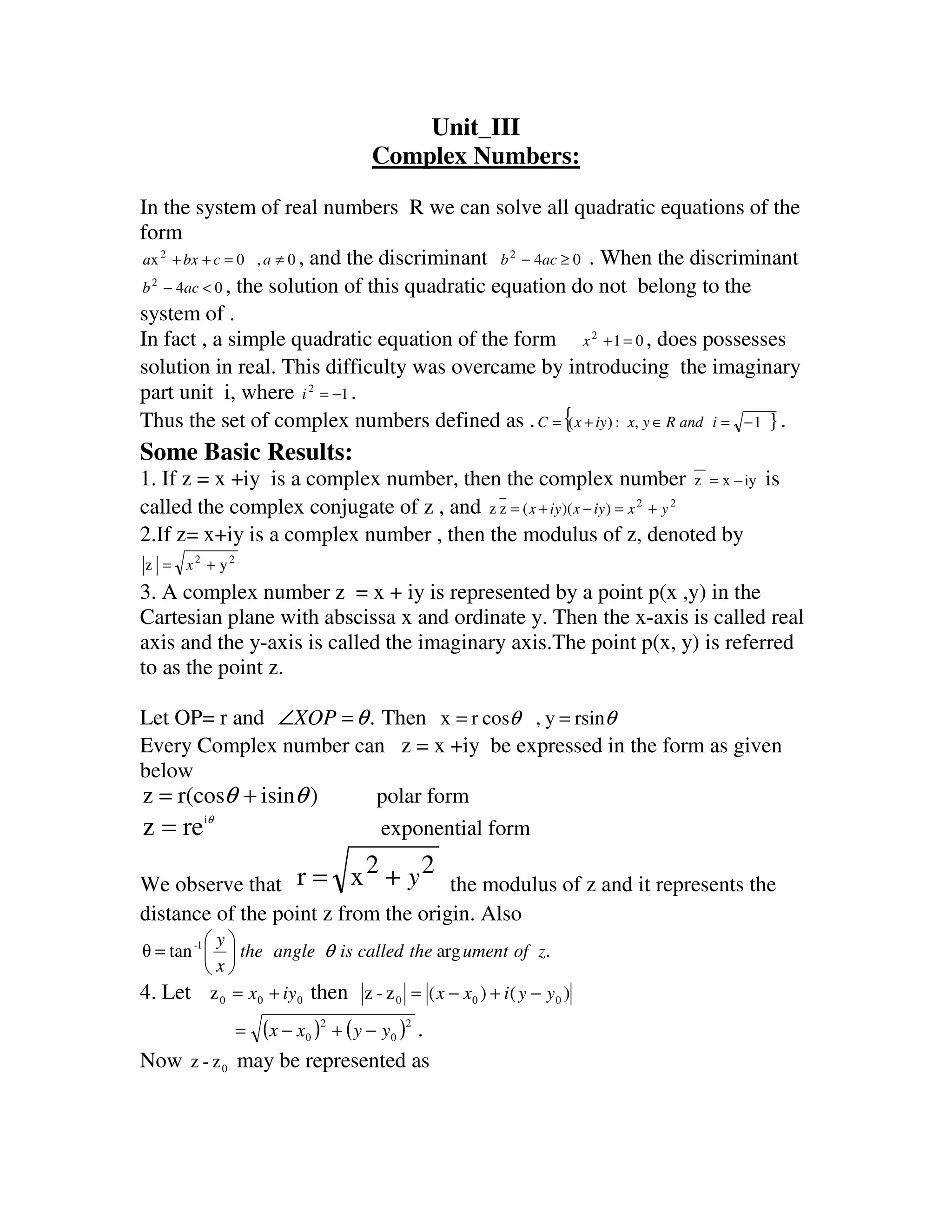
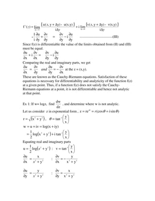
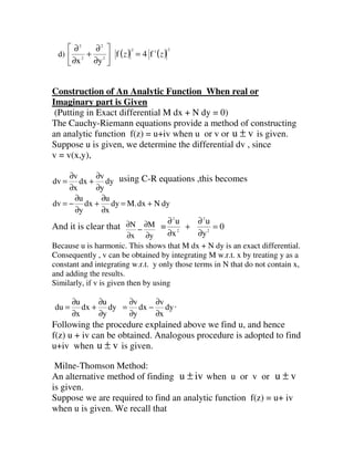
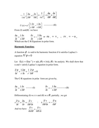
Some different forms of C-R Equations:
If w = f(z) = u+ iv , is analytic , then the following results follows.
1. ( )=z1
f
x
v
i
x
u
∂
∂
+
∂
∂
y
u
i
y
v
∂
∂
−
∂
∂
= 





∂
∂
+
∂
∂
−=
y
v
i
u
i
y
x
v
i
x
u
∂
∂
+
∂
∂
= 





∂
∂
+
∂
∂
−=
y
v
i
u
i
y
y
w
i
x
w
∂
∂
−=
∂
∂
2. ( )
22
21
x
v
x
u
zf 





∂
∂
+





∂
∂
= ( )
22
21
x
v
x
u
zf 





∂
∂
+





∂
∂
=
22
u
x
u






∂
∂
+





∂
∂
=
y
22
x
v






∂
∂
+





∂
∂
=
y
u
using C-R Equations.
Based on the results above mentioned the following results are valid,
a) ( )
2
zf
x 



∂
∂
( )
2
zf
y 





∂
∂
+ ( )
21
f z=
b) ψ is any differential function of x and y then
22
x 





∂
∂
+





∂
∂
y
ψψ
22
vu






∂
∂
+





∂
∂
=
ψψ
( )
21
f z= .
c) 





∂
∂
+
∂
∂
2
2
2
2
yx
( )[ ]2
zfRe ( )
21
f2 z=

9. d) 





∂
∂
+
∂
∂
2
2
2
2
yx
( )2
f z ( )
21
f4 z=
Construction of An Analytic Function When real or
Imaginary part is Given
(Putting in Exact differential M dx + N dy = 0)
The Cauchy-Riemann equations provide a method of constructing
an analytic function f(z) = u+iv when u or v or vu ± is given.
Suppose u is given, we determine the differential dv , since
v = v(x,y),
dy
y
v
dx
x
v
dv
∂
∂
+
∂
∂
= using C-R equations ,this becomes
dyNdxM.dy
x
u
dx
y
u
dv +=
∂
∂
+
∂
∂
−=
And it is clear that
y
M
x
N
∂
∂
−
∂
∂ = 0
y
u
x
u
2
2
2
2
=
∂
∂
+
∂
∂
Because u is harmonic. This shows that M dx + N dy is an exact differential.
Consequently , v can be obtained by integrating M w.r.t. x by treating y as a
constant and integrating w.r.t. y only those terms in N that do not contain x,
and adding the results.
Similarly, if v is given then by using
dy
y
u
dx
x
u
du
∂
∂
+
∂
∂
= dy
x
v
dx
y
v
∂
∂
−
∂
∂
= .
Following the procedure explained above we find u, and hence
f(z) u + iv can be obtained. Analogous procedure is adopted to find
u+iv when vu ± is given.
Milne-Thomson Method:
An alternative method of finding ivu ± when u or v or vu ±
is given.
Suppose we are required to find an analytic function f(z) = u+ iv
when u is given. We recall that

10. 





∂
∂
−
∂
∂
=
y
u
i
x
u
)(f 1
z ------------------------(I)
Let us we set y)x,(
y
u
andy)x,(
x
u
21
φφ =
∂
∂
=
∂
∂
-------(II)
Then y)x,(i)yx,((z)f 21
φφ −=′ --------(III)
Replacing x by z and y by 0, this becomes
z,0)(i)z,0((z)f 21
φφ −=′ -------(IV)
From which the required analytic function f(z) can be got.
Similarly , if v is given we can find the analytic function f(z) = u+ iv by
starting with






∂
∂
+
∂
∂
=
x
v
i
y
v
)(f 1
z Analogous procedure is used when vu ± is given.
Applications to flow problems:
As the real and imaginary parts of an analytic function are the
solutions of the Laplace’s equation in two variable. The conjugate functions
provide solutions to a number of field and flow problems.
Let v be the velocity of a two dimensional incompressible fluid with
irrigational motion, j
y
v
i
x
v
V
∂
∂
+
∂
∂
= ------------------------------(1)
Since the motion is irrotational curl V= 0.
Hence V can be written as
j
y
i
x ∂
∂
+
∂
∂
=∇
φφ
φ -----------------------------(II)
Therefore , φ is the velocity component which is called the velocity
potential. From (I) and (II) we have

11. yy
v
,
xx
v
∂
∂
=
∂
∂
∂
∂
=
∂
∂ φφ
------------------------(III)
Since the fluid is incompressible div V = 0.
0
yyxx
=





∂
∂
∂
∂
+





∂
∂
∂
∂ φφ
-----------------------(IV)
0
yx 2
2
2
2
=
∂
∂
+
∂
∂ φφ
This indicates that φ is harmonic.
The function ( )yx,φ is called the velocity potential , and the curves
( ) cyx, =φ are known as equi -potential lines.
Note : The existence of conjugate harmonic function ( )yx,ψ so that
( ) ( )yx,iyx,w(z) ψφ += is Analytic.
The slope is Given by
x
y
v
v
x
y
y
x
dx
dy
=
∂
∂
∂
∂
=





∂
∂





∂
∂
−=
φ
φ
ψ
ψ
This shows that the velocity of the fluid particle is along the tangent to the
curve ( ) 1
cyx, =ψ , the particle moves along the curve.
( ) 1
cyx, =ψ - is called stream lines ( ) cyx, =φ - called equipotential
lines. As the equipotential lines and stream lines cut orthogonally.
( ) ( )yx,iyx,w(z) ψφ +=
y
i
xx
i
xdz
dw
∂
∂
−
∂
∂
=
∂
∂
+
∂
∂
=
φφψφ
yx
vv −=

12. The magnitude of the fluid velocity ( )
dz
dw
vv 2
y
2
x
=+
The flow pattern is represented by function w(z) known as complex
potential.
Complex potential w(z) can be taken to represent other two-dimensional
problems. (steady flow)
1. In electrostatics ( ) cyx, =φ --- interpreted as equipotential lines.
( ) 1
cyx, =ψ --- interpreted as Lines of force
2. In heat flow problems:
( ) cyx, =φ --- Interpreted as Isothermal lines
( ) 1
cyx, =ψ --- interpreted as heat flow lines.
Cauchy –Riemann equations in polar form:
Let )iv(r,)u(r,)f(ref(z) i
θθθ
+== be analytic at a point z, then
there exists four continuous first order partial derivatives ,
θθ ∂
∂
∂
∂
∂
∂
∂
∂ v
,
r
v
,
u
,
r
u
and satisfy the equations
, .
u
r
1
r
v
:
v1
r
u
θθ ∂
∂
−=
∂
∂
∂
∂
=
∂
∂
r
Proof: The function is analytic at a point
θi
rez = .
z
z
z
∆
−∆+
= →∆
)f(z)f(z
)(f lim0z
1
exists and it is unique.
Now ).iv(r,)u(r,f(z) θθ +=
Let z∆ be the increment in z , corresponding increments are
.andrin,r θθ∆∆

13. { } { }
z
)v(r,i)(r.u)r,(rv),(u
lim)(f
0z
1
∆
+−∆+∆++∆+∆+
=
→∆
θθθθθθ irr
z
{ }
z
)u(r.-),r(ru
lim)(f
0z
1
∆
∆+∆+
=
→∆
θθθ
z
{ }
z
r
∆
∆+∆+
+ →∆
).v(r-),(rv
limi 0z
θθθ
------------------------(I)
Now
θi
rez = and z is a function two variables r and θ , then we have
.
z
r
r
z
z θ
θ
∆
∂
∂
+∆
∂
∂
=∆
( ) ( ) θ
θ
θθ
∆
∂
∂
+∆
∂
∂
=∆ ii
rerre
r
z
θθθ
∆+∆=∆ ii
erirez
When z∆ tends to zero, we have the two following possibilities.
(I). Let rezthatso,0 i
∆=∆=∆ θ
θ
And 0rimplies,0Z →∆→∆
{ }
re
)u(r.-),r(ru
lim)(f i
0r
1
∆
∆+
=
→∆
θ
θθ
z
{ }
re
)v(r.-),(rv
limi i0r
∆
∆+
+ →∆ θ
θθr
The limit exists,




∂
∂
+
∂
∂
= −
r
v
i
r
u
)(f1 θi
ez -----------------(I)
2. Let
θi
erizthatso,0r =∆=∆
And 0imply0,z →∆→∆ θ
{ }
θ
θθθ
θθ
∆
∆+
=
→∆
i
0
1
eri
)u(r.-),(ru
lim)(f z
{ }
θ
θθθ
θ
∆
∆+
+ →∆ i0z
eir
)v(r.-),(rv
limi

14. =




∂
∂
+
∂
∂
θθθ
v
i
u
rei
1
i 



∂
∂
+
∂
∂
−=
θθθ
vu
i
er
1
i




∂
∂
−
∂
∂
=
θθ
θ u
r
iv
r
1
ez)(f i-1
------------ (II)
From (I) and(II) we have
θ∂
∂
=
∂
∂ v
r
1
r
u
θ∂
∂
−=
∂
∂ u
r
1
r
v or θθ
urv,vru rr
−==
Which are the C-R Equations in polar form.
Harmonic Function:
A function φ -is said to be harmonic function if it satisfies Laplace’s
equation 02
=∇ φ
Let )iv(r,)u(r,)f(ref(z) i
θθθ
+== be analytic. We shall show that
u and v satisfy Laplace’s equation in polar form.
0
1
rr
1
r 2
2
22
2
=
∂
∂
+
∂
∂
+
∂
∂
θ
φφφ
r
The C-R equations in polar form are given by,
θ∂
∂
=
∂
∂ v
r
1
r
u ---------(I)
θ∂
∂
−=
∂
∂ u
r
1
r
v ------------(II)
Differentiating (I) w.r.t r and (II) w.r.θ , partially , we get
r
u
r
u
r
2
2
2
∂∂
∂
=
∂
∂
+
∂
∂
θ
v
r
:
2
22
u
r
v
r
θθ ∂
∂
−=
∂∂
∂
And we have
r∂∂
∂
=
∂∂
∂
θθ
v
r
v 22

15. 2
2
2
2
u
r
1
r
u
r
u
r
θ∂
∂
−=
∂
∂
+
∂
∂
Dividing by r we, get
0
u1
r
u
r
1
r
u
2
2
22
2
=
∂
∂
+
∂
∂
+
∂
∂
θr
Hence u-satisfies Laplace’s equation in polar form.
The function is harmonic. Similarly v- is harmonic.
Orthogonal System:
Let )f(r θ= and −= φ
θ
φ ,
dr
d
tan r being the angle between
the radius vector and tangent. The angle between the tangents at
the point of intersection of the curves is 21
φφ − . 1TanTan 21
−=φφ ,is
the condition for orthogonal.
Consider 1
c)u(r, =θ .
Differentiating w.r.t θ , treating r as a function of θ .
0
u
d
dr
r
u
=
∂
∂
+
∂
∂
θθ






∂
∂






∂
∂
−=
r
u
u
d
dr θ
θ
Thus
dr
d
rTan 1
θ
φ = = ( )
( )θ∂
∂
∂
∂
u
r
u
r
=
( )
( )θ∂
∂
∂
∂
u
r
u
r- ---------(I)
Similarly for the curve 2
c)v(r, =θ
=2
Tanφ ( )
( )θ∂
∂
∂
∂
v
r
v
r- -----------(II)

16. ( ) ( )
( ) ( )θθ
φφ
∂
∂
∂
∂
∂
∂
∂
∂
=
vu
r
vr
r
ur
anan 21
TT
By C-R Equations θθ
urv,vru rr
−==
The equation reduces to
( ) ( )
( ) ( ) 1
uv
u-v
anan 21
−=
∂
∂
∂
∂
∂
∂
∂
∂
=
θθ
θθφφTT
Hence the polar family of curves 1
c)u(r, =θ and 2
c)v(r, =θ ,
intersect orthogonally.
Construction of An Analytic Function When real or
Imaginary part is Given(Polar form.)
The method due to Exact differential and Milne-Thomson is
explained in earlier section .
Ex: Verify that ( )θcos2
r
1
u 2
= is harmonic . find also an analytic
function.
Soln: θcos2
r
2
r
u
2






−=
∂
∂ : θ
θ
sin2
r
2u
2






−=
∂
∂
θcos2
r
6
r
u
42
2
=
∂
∂ : θ
θ
cos2
r
4u
22
2
−=
∂
∂ .
Then the Laplace equation in polar form is given by,
=
∂
∂
+
∂
∂
+
∂
∂
2
2
22
2
u1
r
u
r
1
r
u
θr
θcos2
r
6
4
θcos2
r
2
4






− 0cos2
r
4
2
=− θ

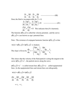
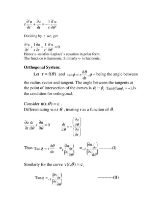
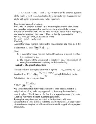
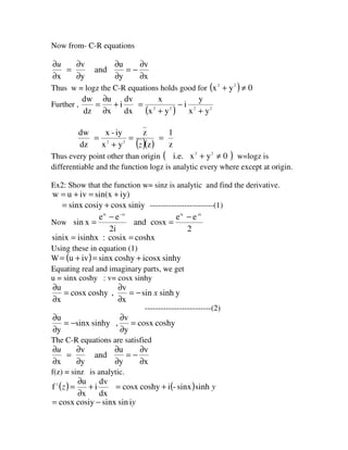
17. Hence u-satisfies the laplace equation and hence is harmonic.
Let us find required analytic function f(z) = u+iv.
We note that from the theory of differentials,
θ
θ
d
v
dr
r
v
dv
∂
∂
+
∂
∂
=
Using C-R equations θθ
urv,vru rr
−==
θ
θ
d
r
u
rdr
u
r
1
- 





∂
∂
+





∂
∂
=
θθθ dcos2
r
2
dsin2
r
2
23






−





−= r






= θsin2
r
1
-d 2
From this csin2
r
1
-v 2
+= θ
c+





+





=+= θθ sin2
r
1
-icos2
r
1
ivuf(z) 22
[ ] icisin2-cos2
r
1
2
+= θθ
( )
ic
er
1
e
r
1
2i
2i-
2
+=+= θ
θ
ic
ic.
z
1
f(z) 2
+=
Ex 2:Find an analytic function f(z)= u+iv given that
θsin
r
1
-rv 





= 0r ≠

18. Soln: θsin
r
1
r
r
v
2






+=
∂
∂ : θ
θ
cos
r
1
r
v






−=
∂
∂
To find u using the differentials
θ
θ
d
u
dr
r
u
du
∂
∂
+
∂
∂
=
Using C-R equations θθ
urv,vru rr
−==
θ
θ
d
r
v
-dr
v
r
1






∂
∂
+





∂
∂
=
θθθ dsin
r
1
1r-drcos
r
1
-r
r
1
2






+





=
= θθθ dsin
r
1
r-drcos
r
1
1 2






+





−












+= θcos
r
1
rd
ccos
r
1
ru +





+= θ
f(z) = u+iv
θθ sin
r
1
-ricos
r
1
r 





++





+= c
( ) cisin-cos
r
1
isinr(cos +++= θθθθ
c
z
1
z
r
1
erf(z) i-i
++=+= θθ
e
Ex: Construction an analytic function given θcos2ru 2
= .
(Milne Thomson Method)

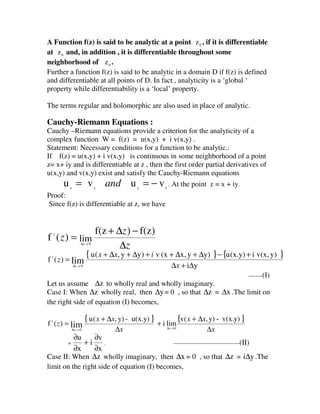
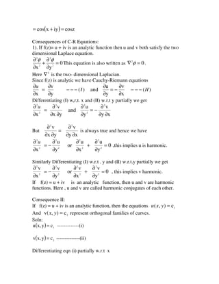
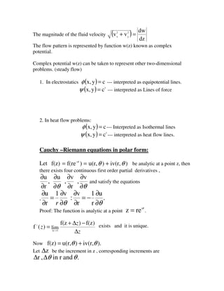
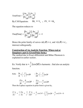
19. θcos2ru 2
= -----------(I)
θ2rcos2
r
u
=
∂
∂
θ
θ
sin22r
u 2
−=
∂
∂




∂
∂
+
∂
∂
= −
r
v
i
r
u
)(f1 θi
ez
Using C-R equations θθ
ur v,vur rr
−==
( ) ( )











+= θθθ
sin22r-
r
1-
ircos22ezf 2i-1
( )[ ]θθθ
sin22rircos22e-i
+=
[ ]θθθ
isin2cos2er2 -i
+=
Now put r = z , and 0=θ .
( ) 2zzf1
= on integrating
( ) czzf 2
+= .
COMPLETION OF UNIT-I