Chapter 9

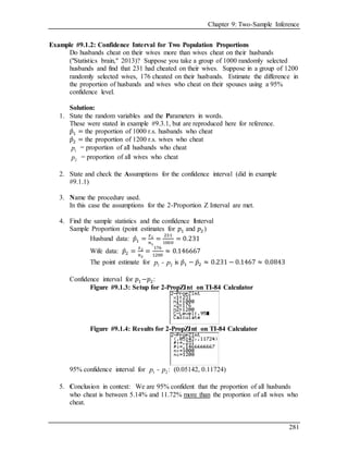
Chapter 9: Two-Sample Inference
276
Chapter 7 discussed methods of hypothesis testing about one population parameter.
Chapter 8 discussed methods of estimating population parameters from one sample using
confidence intervals. This chapter will look at methods of confidence intervals and
hypothesis testing for two populations. Since there are two populations, there are two
random variables, two means or proportions, and two samples (though with paired samples
you usually consider there to be one sample with pairs collected). Some examples of
where you would do this are the following:
 Testing and estimating the difference in testosterone levels of men before and after
they had children (Gettler, McDade, Feranil & Kuzawa, 2011).
 Testing the claim that a diet works by looking at the weight before and after
subjects are on the diet.
 Estimating the difference in proportion of those who approved of President Obama
in the age group 18 to 26-year olds and the 55 and over age group.
All of these are examples of hypothesis tests or confidence intervals for two populations.
The methods to conduct these hypothesis tests and confidence intervals will be explored in
this chapter. As a reminder, all hypothesis tests use the same process (PHANTOMS).
Confidence intervals also all use the same process (PANIC).
Below is a flowchart of where we have been in chapters 7 and 8 and where we are going in
chapter 9. As you can see below, the first most important question to ask is if quantitative
or qualitative information has been collected on each individual object.
Section 9.1 Two Proportions
There are times you want to test a claim about two population proportions or construct a
confidence interval estimate of the difference between two population proportions. As
with all other hypothesis tests and confidence intervals, the process is the same though the
formulas and assumptions are different.

277
Hypothesis Test for Two Population Proportion (2-Prop Z-Test)
1. State the random variables and the Parameters in words.
𝑝̂1 = proportion of 𝑛1 randomly selected objects that are in the category of interest
𝑝1 = proportion of all objects from group 1 that are in the category of interest
2. State the null and alternative Hypotheses and the level of significance
TWO-TAILED TEST LEFT-TAILED TEST RIGHT-TAILED TEST
H0: 𝑝1 = 𝑝2
( 𝑝1 − 𝑝2 = 0)
H 𝐴: 𝑝1 ≠ 𝑝2
( 𝑝1 − 𝑝2 ≠ 0)
H0: 𝑝1 = 𝑝2
( 𝑝1 − 𝑝2 = 0)
H 𝐴: 𝑝1 < 𝑝2
( 𝑝1 − 𝑝2 < 0)
H0: 𝑝1 = 𝑝2
( 𝑝1 − 𝑝2 = 0)
H 𝐴: 𝑝1 > 𝑝2
( 𝑝1 − 𝑝2 > 0)
Also, state your 𝛼 level here.
3. State and check the Assumptions for a hypothesis test
a. A simple random sample of size 𝑛1 is taken from population 1, and a simple random
sample of size 𝑛2 is taken from population 2.
b. The samples are independent.
c. There are only two categories for each object (same for both samples)
d. There are at least 10 objects in each category for both sets of sample data
This means 𝑥1, 𝑛1 − 𝑥1, 𝑥2, 𝑛2 − 𝑥2 are all at least 10
e. 𝑁1 ≥ 20𝑛1 and 𝑁2 ≥ 20𝑛2 (Assume true if population sizes are not given)
4. Name the test used: In this case the assumptions for the 2-Proportion ZTest have been met
5. Find the sample statistics and Test statistic
Sample Proportions:
𝑝̂1 =
𝑥1
𝑛1
= proportion of successes in sample 1
𝑝̂2 =
𝑥2
𝑛2
Pooled Sample Proportion, 𝑝̂:
𝑝̂ =
𝑥1+𝑥2
𝑛1+𝑛2
Test Statistic:
𝑧 =
(𝑝̂1−𝑝̂2)
√(𝑝̂(1−𝑝̂)(
1
𝑛1
+
1
𝑛2
))
(you can get this final value off the output screen)
6. Obtain the p-value and illustrate the meaning of the p-value, sample statistic and test statistic.
Using the TI84: Use 2-PropZTest from the STAT TESTS menu
𝑝̂1 − 𝑝̂2 :
z:
𝑝̂1 − 𝑝̂2 :
z:
𝑝̂1 − 𝑝̂2 :
z:
Using StatCrunch: Use Stat, Proportion Stats,Two Sample, With Summary
7. Make a decision about H0
Reject 𝐻0 if the p-value ≤ a and fail to reject 𝐻0 if the p-value > a
8. State a conclusion in the context of the problem
 If you reject 𝐻0, then there is significant evidence to conclude (𝐻𝐴 in context)
 If you fail to reject 𝐻0, then there is NOT significant evidence to conclude (𝐻𝐴 in context)

278
Confidence Interval for the Difference between Two Population
Proportions (2-Prop Z Interval)
2. State and check the Assumptions.
a. A simple random sample of size 𝑛1 is taken from population 1, and a simple random
sample of size 𝑛2 is taken from population 2.
b. The samples are independent.
c. There are only two categories for each object (same for both samples)
d. There are at least 10 objects in each category for both sets of sample data
This means 𝑥1, 𝑛1 − 𝑥1, 𝑥2, 𝑛2 − 𝑥2 are all at least 10
e. 𝑁1 ≥ 20𝑛1 and 𝑁2 ≥ 20𝑛2 (Assume true if population sizes are not given)
3. Name the procedure used.
In this case the assumptions for 2-Proportion Z Interval have been met.
4. Find the point estimate and the Interval estimate
Using the TI84: Go to STAT TESTS and use 2-Proportion Z Interval
Using StatCrunch: Use Stat, Proportion Stats,2 Sample, With Summary
Sample Proportions:
𝑝̂1 =
𝑥1
𝑛1
𝑝̂2 =
𝑥2
𝑛2
𝑝̂1 − 𝑝̂2 =
𝑥1
𝑛1
−
𝑥2
𝑛2
Confidence Interval for p1 – p2: This interval is given in the output of the technology
5. Conclusion in context: In general, if you convert the endpoints from proportions to percentages,
this looks like one of the following:
 If both endpoints are positive: “We are C% confident that the percentage of all objects
from population 1 that are in the category of interest exceeds the percentage of all
objects from population 2 that are in the category of interest by a percentage between
lower endpoint and upper endpoint.”
 If both endpoints are negative: “We are C% confident that the percentage of all
objects from population 1 that are in the category of interest is less than the percentage
of all objects from population 2 that are in the category of interest by a percentage
between |upper endpoint| and |lower endpoint|.”
o Be careful not to have negative percentages here
 If one endpoint is negative and one endpoint is positive, then you do not have any
evidence of a difference in the groups.
One way to compare two values is to subtract them and see the difference. Although the order of
this subtraction gives you a different sign for your answer,it does not give you a different answer
when you include the context. For example, let’s say that I have $10 and you have $4.
 If we take $10 - $4 = $6, this means that I have 6 dollars more than you do.
 If we take $4 - $10 = -$6, then means that you have 6 dollars less than I do.

279
Example #9.1.1: Hypothesis Test for Two Population Proportions
Do husbands cheat on their wives more than wives cheat on their husbands
("Statistics brain," 2013)? Suppose you take a group of 1000 randomly selected
husbands and find that 231 had cheated on their wives. Suppose in a group of 1200
randomly selected wives, 176 cheated on their husbands. Do the data show that the
proportion of husbands who cheat on their wives are more than the proportion of
wives who cheat on their husbands. Test at the 5% level.
Solution:
𝑝̂1 = the proportion of 1000 r.s. husbands who cheat
𝑝̂2 = the proportion of 1200 r.s. wives who cheat
p1
= proportion of all husbands who cheat
p2
= proportion of all wives who cheat
Ho : p1 = p2
or Ho : p1 - p2 = 0
HA : p1 > p2 HA : p1 - p2 > 0
a = 0.05
a. A simple random sample of 1000 responses about cheating from husbands is
taken. This was stated in the problem. A simple random sample of 1200
responses about cheating from wives is taken. This was stated in the problem.
b. The samples are independent since each sample was randomly selected so there
are probably not any husband and wife pairs in the group.
c. Each person in the study either cheated on their spouse or they didn’t
d. x1 = 231, n1 - x1 =1000 - 231= 769, x2 =176, and
n2 - x2 =1200 -176 =1024 are all greater than or equal to 10.
e. No population sizes were given so we will assume 𝑁1 ≥ 20𝑛1 and 𝑁2 ≥ 20𝑛2
4. Name the test used
In this case the assumptions for the 2-Proportion Z Test are met
On TI-84: Use 2-PropZTest in the STAT TESTS menu
Figure #9.1.1: Setup for 2-PropZTest on TI-84 Calculator

280
Figure #9.1.2: Results for 2-PropZTest on TI-84 Calculator
Using StatCrunch: Use Stat, Proportion Stats, 2 Sample, With Summary
No matter what technology you use, you get the following:
Sample Proportions:
Husband data: 𝑝̂1 =
𝑥1
𝑛1
=
231
1000
= 0.231
Wife data: 𝑝̂2 =
𝑥2
𝑛2
=
176
1200
≈ 0.146667
𝑝̂1 − 𝑝̂2 =
231
1000
−
176
1200
≈ 0.084333
Pooled Sample Proportion, 𝑝̂:
𝑝̂ =
231+176
1000+1200
=
407
2200
= 0.185
Test Statistic: The final value is on the output of the 2-PropZTest screen
𝑧 =
(𝑝̂1−𝑝̂2)
√(𝑝̂(1−𝑝̂)( 1
𝑛1
+
1
𝑛2
))
=
( 231
1000
−
176
1200
)
√( 407
2200
(1−
407
2200
)( 1
1000
+
1
1200
))
≈ 5.0724
6. Obtain the p-value and illustrate the meaning of the p-value, sample statistic and
test statistic.
On the TI84, you get p-value ≈ 1.96 × 10−7
. On StatCrunch you get p-value <
0.001.
7. Make a decision about 𝐻0
Reject 𝐻0, since the p-value is less than or equal to 5%.
8. State a conclusion in the context of the problem.
This is significant evidence to conclude that the proportion of all husbands who
cheat is more than the proportion of all wives who cheat.
In the hypothesis test above, we concluded that the proportion of all husbands who cheat is
more than the proportion of all wives who cheat. A next question someone might ask is
how much more? That can be answered with a confidence interval for the difference in
two population proportions.

281
Example #9.1.2: Confidence Interval for Two Population Proportions
Do husbands cheat on their wives more than wives cheat on their husbands
("Statistics brain," 2013)? Suppose you take a group of 1000 randomly selected
husbands and find that 231 had cheated on their wives. Suppose in a group of 1200
randomly selected wives, 176 cheated on their husbands. Estimate the difference in
the proportion of husbands and wives who cheat on their spouses using a 95%
confidence level.
Solution:
These were stated in example #9.3.1, but are reproduced here for reference.
𝑝̂1 = the proportion of 1000 r.s. husbands who cheat
𝑝̂2 = the proportion of 1200 r.s. wives who cheat
p1
= proportion of all husbands who cheat
p2
= proportion of all wives who cheat
2. State and check the Assumptions for the confidence interval (did in example
#9.1.1)
In this case the assumptions for the 2-Proportion Z Interval are met.
4. Find the sample statistics and the confidence Interval
Sample Proportion (point estimates for 𝑝1 and 𝑝2)
Husband data: 𝑝̂1 =
𝑥1
𝑛1
=
231
1000
= 0.231
Wife data: 𝑝̂2 =
𝑥2
𝑛2
=
176
1200
≈ 0.146667
The point estimate for p1 - p2
is 𝑝̂1 − 𝑝̂2 ≈ 0.231 − 0.1467 ≈ 0.0843
Confidence interval for 𝑝1−𝑝2:
Figure #9.1.3: Setup for 2-PropZInt on TI-84 Calculator
Figure #9.1.4: Results for 2-PropZInt on TI-84 Calculator
95% confidence interval for p1 - p2
: (0.05142, 0.11724)
5. Conclusion in context: We are 95% confident that the proportion of all husbands
who cheat is between 5.14% and 11.72% more than the proportion of all wives who
cheat.

282
Section9.1:Homework
In each problem show all steps of the hypothesis test (PHANTOMS) or confidence interval
(PANIC). If some of the assumptions are not met, note that the results of the test or
interval may not be correct and then continue the process of the hypothesis test or
confidence interval.
1.) Many high school students take the AP tests in different subject areas. In 2007, of
the 144,796 students who took the biology exam 84,199 of them were female. In
that same year, of the 211,693 students who took the calculus AB exam 102,598 of
them were female ("AP exam scores," 2013). Is there enough evidence to show
that the proportion of AP biology exam takers who are female is higher than the
proportion of AP calculus AB exam takers who are female? Test at the 5% level.
the 144,796 students who took the biology exam 84,199 of them were female. In
that same year, of the 211,693 students who took the calculus AB exam 102,598 of
them were female ("AP exam scores," 2013). Estimate the difference in the
proportion of AP biology exam takers who are female and the proportion of AP
calculus AB exam takers who are female using a 90% confidence level.
the 211,693 students who took the calculus AB exam 102,598 of them were female
and 109,095 of them were male ("AP exam scores," 2013). Is there enough
evidence to show that the proportion of AP calculus AB exam takers who are
female is different from the proportion of AP calculus AB exam takers who are
male? Test at the 5% level.
the 211,693 students who took the calculus AB exam 102,598 of them were female
and 109,095 of them were male ("AP exam scores," 2013). Estimate the difference
between the proportion of AP calculus AB exam takers who are female and the
proportion of AP calculus AB exam takers who are male using a 90% confidence
level.
5.) Are there less children diagnosed with Autism Spectrum Disorder (ASD) in states
that have larger urban areas over states that are mostly rural? In the state of
Pennsylvania, a fairly urban state, there are 245 eight-year olds diagnosed with
ASD out of 18,440 eight-year olds evaluated. In the state of Utah, a fairly rural
state, there are 45 eight-year olds diagnosed with ASD out of 2,123 eight-year olds
evaluated ("Autism and developmental," 2008). Is there enough evidence to show
that the proportion of children diagnosed with ASD in Pennsylvania is less than the
proportion in Utah? Test at the 1% level.

283
6.) Are there more children diagnosed with Autism Spectrum Disorder (ASD) in states
that have larger urban areas over states that are mostly rural? In the state of
Pennsylvania, a fairly urban state, there are 245 eight-year olds diagnosed with
ASD out of 18,440 eight-year olds evaluated. In the state of Utah, a fairly rural
state, there are 45 eight-year olds diagnosed with ASD out of 2,123 eight-year olds
evaluated ("Autism and developmental," 2008). Estimate the difference in
proportion of children diagnosed with ASD between Pennsylvania and Utah. Use a
98% confidence level.
7.) A child dying from an accidental poisoning is a terrible incident. Is it more likely
that a male child will get into poison than a female child? To find this out, data
were collected that showed that out of 1830 children between the ages one and four
who pass away from poisoning, 1031 were males and 799 were females (Flanagan,
Rooney & Griffiths, 2005). Do the data show that there are more male children
dying of poisoning than female children? Test at the 1% level.
8.) A child dying from an accidental poisoning is a terrible incident. Is it more likely
that a male child will get into poison than a female child? To find this out, data
were collected that showed that out of 1830 children between the ages one and four
who pass away from poisoning, 1031 were males and 799 were females (Flanagan,
Rooney & Griffiths, 2005). Compute a 99% confidence interval for the difference
in proportions of poisoning deaths of male and female children ages one to four.

284
Section 9.2 Paired Samples for Two Means
Are two populations the same? Is the average height of men taller than the average height
of women? Is the mean weight less after a diet than before?
When quantitative data have been collected, you can compare populations by comparing
their means. You take a sample from each population and compare the statistics.
Anytime you compare two populations you need to know if the samples are independent or
dependent. The formulas you use are different for different types of samples.
Dependent (or Matched Pairs) Samples – Samples that have been matched based on
some criteria or samples in which the 2 measurements were taken on the same object,
one before and one after some particular treatment. Here the individuals in one sample
dictate the individuals in the second sample.
 We have two values of the same variable recorded for the same or similar object
Independent Samples – when the individuals in one sample do not dictate which
individuals are to be in the second sample.
 We have two values of the same variable recorded for two different objects that
have not been matched or paired together in any way.
Example #9.2.1: Independent or Dependent Samples
Determine if the following are dependent or independent samples.
a.) Randomly choose 5 men and 6 women and measure their heights
Solution:
The individuals are not the same for both samples and the 5 men have not been
paired on any criteria with the 6 women. So these samples are independent.
b.) Choose 10 men and weigh them. Give them a new wonder diet drug and later
weigh them again.
Solution:
Each person’s before weight can be matched with their after weight. In this case
we have two measurements of weight on the same person. So these samples are
dependent.
c.) Take 10 people and measure the strength of their dominant arm and their non-
dominant arm.
Solution:
In this case we have two measurements of strength on the same person. Although
the measurements are for different arms, how strong a person is with one arm will
depend on how strong they are with the other. So these samples are dependent.

285
To analyze data when there are dependent samples, we will start by entering two lists of
paired data and then computing a list of differences.
TECHNOLOGY: COMPUTING A LIST OF DIFFERENCES
Using StatCrunch:
 Enter the two lists of data in the spreadsheet
 Click Data, Compute, Expression
 In the popup window that opens type the expression “var1” – “var2” where you
would specifically put the names of those variables inside of the quotation marks.
Below the expression is “After” – “Before”
 Then click “Compute!”
 You will see a new column added to the spreadsheet and all of the differences have
been computed for you where each difference, d, is computed as 𝑑 = 𝑥1 − 𝑥2
Using your TI84:
 First push STAT 1 and enter the data into L1 and L2
 Use the arrow keys to highlight L3 and then type "L1 – L2" by pushing 2nd 1 − 2nd
2
 Then push ENTER
 L3 will now have all of the computed differences.
 NOTE: If you get “ERR: DATA TYPE”, then you did not have your cursor above
the line highlighting L3 before you entered L1-L2

286
Hypothesis Test for Paired T-Test (T-Test on differences)
Before starting,you need to enter the two lists of paired data and compute the list of differences. (see
instructions on previous page)
X̅1 = the mean measurement of 𝑛1 randomly selected objects from group 1
𝜇1 = mean measurement of all objects in group 1 (usually an after measurement)
𝜇2 = mean measurement of all objects in group 2 (usually a before measurement)
For this paired test, 𝜇 𝑑 = 𝜇1 − 𝜇2 = the mean difference in the measurements of all objects
H0: 𝜇 𝑑 = 0
H 𝐴: 𝜇 𝑑 ≠ 0
H0: 𝜇 𝑑 = 0
H 𝐴: 𝜇 𝑑 < 0
H0: 𝜇 𝑑 = 0
H 𝐴 : 𝜇 𝑑 > 0
a) A simple random sample of size n is taken from each group.
b) The sample are dependent (paired)
c) Normal population of differences or at least 30 pairs of data with no outliers in the
differences
 Use the techniques from chapter 6 to assess normality. The modified boxplot needs
to showno outliers. If the sample is less than 30, you also need the normal
probability plot to be roughly linear.
d) Population standard deviation is unknown for each group
4. Name the test used: In this case,the assumptions for the Paired TTest have been met
Sample Differences:
𝑑̅ =
𝑠𝑢𝑚 𝑜𝑓 𝑑𝑖𝑓𝑓𝑒𝑟𝑒𝑛𝑐𝑒 𝑙𝑖𝑠𝑡
𝑛
, this is next to 𝑥̅ on the output screen
(𝑠 𝑑 is also on the output screen next to 𝑠 𝑥)
Test Statistic:
t=
( 𝑑̅−𝜇 𝑑
)
(
𝑠 𝑑
√𝑛
)
=
𝑑̅
(
𝑠 𝑑
√𝑛
)
In this class, 𝜇 𝑑 will always be 0.
Use TTest from the STAT TESTS menu. Use the list of differences and enter 0 next to 𝜇0
The p-value is next to “p” on the output screen,but you need to write “p-value = “
𝑑̅:
t:
𝑑̅:
t:
𝑑̅:
t:

287
Confidence Interval for the Differences in Means from Paired
Samples (T Interval on List of Differences)
Before starting,you need to enter the two lists of paired data and compute the list of differences. (see
earlier instructions)
𝜇1 = mean measurement of all objects in group 1 (usually an after measurement)
𝜇2 = mean measurement of all objects in group 2 (usually a before measurement)
2. State and check the Assumptions.
a) A simple random sample of size n is taken from each group
b) The samples are dependent (paired)
c) Normal population of differences or at least 30 pairs of data with no outliers in the
differences
 Use the techniques from chapter 6 to assess normality. The modified boxplot
needs to show no outliers. If the sample is less than 30, you also need the normal
In this case the assumptions for Paired T Interval have been met.
Sample differences:
𝑑̅ =
𝑠𝑢𝑚 𝑜𝑓 𝑑𝑖𝑓𝑓𝑒𝑟𝑒𝑛𝑐𝑒 𝑙𝑖𝑠𝑡
𝑛
, this is next to 𝑥̅ on the output screen
Confidence Interval for 𝜇 𝑑:
On the TI84: Use T Interval on the list of differences
 The confidence interval is given at the top of the output screen
 The value of 𝑑̅ and 𝑠 𝑑 are next to 𝑥̅ and 𝑠 𝑥 respectively
Using StatCrunch: Use Stat, T Tests, Paired. Then select the columns and enter a
confidence level, and then click “Compute!”
You can also do Stat, T Tests,One Sample, With Data on the list of differences
 The value of 𝑑̅ is under the column called “Sample Mean” and the interval
endpoints are under the columns “L. Limit” and “U. Limit”
 The number under “Std. Err” is
𝑠 𝑑
√𝑛
which is why it does not match the standard
deviation given by the TI84 which is the value of 𝑠 𝑑
5. Conclusion in context:
 If both endpoints are positive: “We are C% confident that the mean measurement of
all objects in group 1 exceeds the mean measurement of all objects in group 2 by an
amount between lower endpoint and upper endpoint.”
 If both endpoints are negative: “We are C% confident that the mean measurement of
all objects in group 1 is less than the mean measurement of all objects in group 2 by an
amount between |upper endpoint|and |lower endpoint|.”
o Be careful not to have negative numbers here

288
Example #9.2.2: Hypothesis Test for Paired Samples Using Technology
The New Zealand Air Force purchased a batch of flight helmets. They then found
out that the helmets didn’t fit. In order to make sure that they order the correct size
helmets, they measured the head size of recruits. To save money, they wanted to
use cardboard calipers, but were not sure if they will be accurate enough. So they
took 18 recruits and measured their heads with the cardboard calipers and also with
metal calipers. The data in centimeters (cm) are in table #9.2.3 ("NZ helmet size,"
2013). Do the data provide enough evidence to show that there is a difference in
measurements between the cardboard and metal calipers? Use a 5% level of
significance.
Table #9.2.1: Data for Head Measurements
Metal 145 153 161 151 145 150 150 163 147 154 150 156 161 152 154 154 147 160
Cardboard 146 151 163 152 151 151 149 166 149 155 155 156 162 150 156 158 149 163
Solution:
X̅1 = the mean head size of 18 r.s. recruits using a metal caliper
X̅2 = the mean head size of 18 r.s. recruits using a cardboard caliper
m1
= the mean head size of all recruits using a metal caliper
m2
= the mean head size of all recruits using a cardboard caliper
Ho :md = 0
HA :md ¹ 0
a = 0.05
(Since is stated that we wanted to test for a difference)
3. State and check the Assumptions for the hypothesis test
a. A random sample of 18 pairs of head measures of recruits with cardboard
and metal caliper was taken.
b. Two measurements were taken on each recruit so this is paired data
(dependent samples)
c. The population of the difference in head measurements between cardboard
and metal calipers is normally distributed or we have at least 30 pairs of
data. We only have 18 pairs of data, so we need to see if the differences are
normally distributed by looking at the histogram, modified boxplot, and the
normal probability plot.
 These are paired data so you should put the data into L1 and L2 and a
difference list in L3 = L1 – L2. The histogram, modified boxplot and
normal probability plot are made with L3

289
Figure #9.2.1: Histogram of Differences in Head Sizes
This histogram looks roughly bell shaped.
Figure #9.2.2: Modified Box Plot of Differences in Head Sizes
There are no outliers in the difference data set.
Figure #9.2.3: Normal Probability Plot of Differences in Head Sizes
The normal probability plot on the differences looks somewhat linear.
So you can assume that the distribution of the difference in weights is normal.
d. The population standard deviation is not known for either group.
 These values were not given and we cannot compute population
standard deviations from sample data.

290
4. Name the test used: In this case, the assumptions for the Paired TTest have
been met
5. Find the sample statistic and Test statistic
Using the TI-84: You would first need to enter both lists of data and compute
the difference list in L3 as L1 – L2. Then under STAT TESTS use T-Test as
shown in figure #9.2.4
Figure #9.2.4: Setup for T-Test on TI-84 Calculator
Once you press ENTER on Calculate you will see the result shown in figure
#9.2.5.
Figure #9.2.5: Results of T-Test on TI-84 Calculator
Using StatCrunch: Use Stat, T Tests, One Sample, With Data using the list of
differences (or you can use Stat, T Tests, Paired and choose the two lists)
No matter what technology you use, you get the following results:
Sample difference: 𝑑̅ ≈ −1.611111 cm
 This does not mean that someone had a -1.61 cm head size!
 In this problem d = metal measurement – cardboard measurement
So this means that the mean measurement with the metal caliper was
about 1.61 cm less than the mean measurement with the cardboard
calipers.
Test statistic:
𝑡 =
𝑑̅−𝜇 𝑑
𝑠 𝑑/√ 𝑛
≈
−1.611111−0
2.145827
√18
≈ −3.19
 This means that the observed mean difference is about 3.19 standard
deviations below the claimed mean difference of 0.

291
6. Obtain the p-value and illustrate the meaning of the p-value, sample statistic
and test statistic.
From the screen above, the p-value ≈ 0.0054
This is a two-tailed test, so the p-value will be the area in two tails. Use
symmetry to get the other values on the axis.
7. Make a conclusion about 𝐻0
Since the p-value ≤ 0.05, reject 𝐻0.
8. State a conclusion in context.
There is enough evidence to show that the mean of all head measurements
using the metal calipers differs from the mean of all head measurements when
using the cardboard calipers. So it looks like the New Zealand Air Force
shouldn’t use the cardboard calipers.
Example #9.2.3: Confidence Interval for Paired Samples Using Technology
The New Zealand Air Force purchased a batch of flight helmets. They then found
out that the helmets didn’t fit. In order to make sure that they order the correct size
helmets, they measured the head size of recruits. To save money, they wanted to
use cardboard calipers, but were not sure if they will be accurate enough. So they
took 18 recruits and measured their heads with the cardboard calipers and also with
metal calipers. The data in centimeters (cm) are in table #9.2.3 ("NZ helmet size,"
2013). Estimate the mean difference in measurements between the cardboard and
metal calipers using a 95% confidence interval.
Solution:
X̅1 = the mean head size of 18 r.s. recruits using a metal caliper
X̅2 = the mean head size of 18 r.s. recruits using a cardboard caliper
m1
= the mean head size of all recruits using a metal caliper
m2
= the mean head size of all recruits using a cardboard caliper
The assumptions were stated and checked in example #9.2.2.
3. Name the procedure used
In this case the assumptions for the Paired T Interval are met.

292
4. Find the sample statistic and confidence Interval
Using the TI-84, You would first need to enter both lists of data and compute
the difference list in L3 as L1 – L2. Then under STAT TESTS Then chose
TInterval. The setup for the calculator is in figure #9.2.6.
Figure #9.2.6: Setup for TInterval on TI-84 Calculator
Once you press ENTER on Calculate you will see the result shown in figure
#9.2.7.
Figure #9.2.7: Results of TInterval on TI-84 Calculator
Point estimate for 𝜇 𝑑 is 𝑑̅ ≈ −1.611 𝑐𝑚
95% confidence interval for 𝜇 𝑑 is (-2.678 cm, -0.544 cm)
5. Conclusion in context: We are 95% confident that the mean head measurement
of all recruits using the metal caliper is between 0.54 cm and 2.68 cm less than
the mean head measurement of all recruits using the cardboard calipers.
NOTE: If you had subtracted your lists as L2 – L1, you would have gotten the following
interval: (0.544 cm, 2.678 cm). In this case we would say we are 95% confident that the
mean head measurement of all recruits using the cardboard caliper is between 0.54 cm and
2.68 cm more than the mean head measurement of all recruits using the metal calipers.
So although we would have gotten different signs on the answers, the interpretations mean
the same thing.
Examples #9.2.2 and #9.2.3 use the same data set, but one is conducting a hypothesis test
and the other is conducting a confidence interval. If you want to show that the means are
different, then conduct a hypothesis test. If you want to estimate the mean difference, then
conduct a confidence interval.

293
Section9.2:Homework
In each problem show all steps of the hypothesis test (PHANTOMS) or confidence interval
(PANIC). If some of the assumptions are not met, note that the results of the test or
interval may not be correct and then continue the process of the hypothesis test or
confidence interval.
1.) The cholesterol level of patients who had heart attacks was measured two days after
the heart attack and then again four days after the heart attack. The researchers
want to see if the cholesterol level of patients who have heart attacks reduces as the
time since their heart attack increases. The data is in table #9.2.4 ("Cholesterol
levels after," 2013). Do the data show that the mean cholesterol level of patients
that have had a heart attack reduces as the time increases since their heart attack?
Test at the 1% level.
Table #9.2.4: Cholesterol Levels (in mg/dL) of Heart Attack Patients
Patient Cholesterol
Level Day
2
Cholesterol
Level Day
4
1 270 218
2 236 234
3 210 214
4 142 116
5 280 200
6 272 276
7 160 146
8 220 182
9 226 238
10 242 288
11 186 190
12 266 236
13 206 244
14 318 258
15 294 240
16 282 294
17 234 220
18 224 200
19 276 220
20 282 186
21 360 352
22 310 202
23 280 218
24 278 248
25 288 278
26 288 248
27 244 270
28 236 242

294
2.) The cholesterol level of patients who had heart attacks was measured two days after
the heart attack and then again four days after the heart attack. The researchers
want to see if the cholesterol level of patients who have heart attacks reduces as the
time since their heart attack increases. The data is in table #9.2.4 ("Cholesterol
levels after," 2013). Calculate a 98% confidence interval for the mean difference in
cholesterol levels from day two to day four.
3.) All Fresh Seafood is a wholesale fish company based on the east coast of the U.S.
Catalina Offshore Products is a wholesale fish company based on the west coast of
the U.S. Table #9.2.5 contains prices from both companies for specific fish types
("Seafood online," 2013) ("Buy sushi grade," 2013). Do the data provide enough
evidence to show that a west coast fish wholesaler is more expensive than an east
coast wholesaler? Test at the 5% level.
Table #9.2.5: Wholesale Prices of Fish in Dollars
Fish
All Fresh
Seafood
Prices
Catalina
Offshore
Products Prices
Cod 19.99 17.99
Tilapi 6.00 13.99
Farmed Salmon 19.99 22.99
Organic Salmon 24.99 24.99
Grouper Fillet 29.99 19.99
Tuna 28.99 31.99
Swordfish 23.99 23.99
Sea Bass 32.99 23.99
Striped Bass 29.99 14.99
4.) All Fresh Seafood is a wholesale fish company based on the east coast of the U.S.
Catalina Offshore Products is a wholesale fish company based on the west coast of
the U.S. Table #9.2.5 contains prices from both companies for specific fish types
("Seafood online," 2013) ("Buy sushi grade," 2013). Find a 95% confidence
interval for the mean difference in wholesale price between the east coast and west
coast suppliers.

295
5.) The British Department of Transportation studied to see if people avoid driving on
Friday the 13th. They did a traffic count on a Friday and then again on a Friday the
13th at the same two locations ("Friday the 13th," 2013). The data for each location
on the two different dates is in table #9.2.6. Do the data show that on average
fewer people drive on Friday the 13th? Test at the 5% level.
Table #9.2.6: Traffic Count
Dates 6th 13th
1990, July 139246 138548
1990, July 134012 132908
1991, September 137055 136018
1991, September 133732 131843
1991, December 123552 121641
1991, December 121139 118723
1992, March 128293 125532
1992, March 124631 120249
1992, November 124609 122770
1992, November 117584 117263
6.) The British Department of Transportation studied to see if people avoid driving on
Friday the 13th. They did a traffic count on a Friday and then again on a Friday the
13th at the same two locations ("Friday the 13th," 2013). The data for each location
on the two different dates is in table #9.2.6. Estimate the mean difference in traffic
count between the 6th and the 13th using a 90% level.

296
7.) To determine if Reiki is an effective method for treating pain, a pilot study was
carried out where a certified second-degree Reiki therapist provided treatment on
volunteers. Pain was measured using a visual analogue scale (VAS) immediately
before and after the Reiki treatment (Olson & Hanson, 1997). The data is in table
#9.2.7. Do the data show that Reiki treatment reduces pain? Test at the 5% level.
Table #9.2.7: Pain Measures Before and After Reiki Treatment
VAS
before
VAS
after
6 3
2 1
2 0
9 1
3 0
3 2
4 1
5 2
2 2
3 0
5 1
1 0
6 4
6 1
4 4
4 1
7 6
2 1
4 3
8 8
8.) To determine if Reiki is an effective method for treating pain, a pilot study was
carried out where a certified second-degree Reiki therapist provided treatment on
volunteers. Pain was measured using a visual analogue scale (VAS) immediately
before and after the Reiki treatment (Olson & Hanson, 1997). The data is in table
#9.2.7. Compute a 90% confidence level for the mean difference in VAS score
from before and after Reiki treatment.

297
9.) The female labor force participation rates (FLFPR) of women in randomly selected
countries in 1990 and latest years of the 1990s are in table #9.2.8 (Lim, 2002). Do
the data show that the mean female labor force participation rate in 1990 is
different from that in the latest years of the 1990s using a 5% level of significance?
Table #9.2.8: Female Labor Force Participation Rates
Region and country
FLFPR
25-54
1990
FLFPR
25-54
Latest year of
1990s
Iran 22.6 12.5
Morocco 41.4 34.5
Qatar 42.3 46.5
Syrian Arab Republic 25.6 19.5
United Arab Emirates 36.4 39.7
Cape Verde 46.7 50.9
Ghana 89.8 90.0
Kenya 82.1 82.6
Lesotho 51.9 68.0
South Africa 54.7 61.7
Bangladesh 73.5 60.6
Malaysia 49.0 50.2
Mongolia 84.7 71.3
Myanmar 72.1 72.3
Argentina 36.8 54
Belize 28.8 42.5
Bolivia 27.3 69.8
Brazil 51.1 63.2
Colombia 57.4 72.7
Ecuador 33.5 64
Nicaragua 50.1 42.5
Uruguay 59.5 71.5
Albania 77.4 78.8
Uzbekistan 79.6 82.8
10.) The female labor force participation rates of women in randomly selected countries
in 1990 and latest years of the 1990s are in table #9.2.8 (Lim, 2002). Estimate the
mean difference in the female labor force participation rate in 1990 to latest years
of the 1990s using a 95% confidence level?

298
11.) Table #9.2.9 contains pulse rates collected from males, who are non-smokers but
do drink alcohol ("Pulse rates before," 2013). The before pulse rate is before they
exercised, and the after pulse rate was taken after the subject ran in place for one
minute. Do the data indicate that the pulse rate before exercise is less than after
exercise? Test at the 1% level.
Table#9.2.9: Pulse Rate of Males Before and After Exercise
Pulse
before
Pulse
after
76 88
56 110
64 126
50 90
49 83
68 136
68 125
88 150
80 146
78 168
59 92
60 104
65 82
76 150
145 155
84 140
78 141
85 131
78 132
12.) Table #9.2.9 contains pulse rates collected from males, who are non-smokers but
do drink alcohol ("Pulse rates before," 2013). The before pulse rate is before they
exercised, and the after pulse rate was taken after the subject ran in place for one
minute. Compute a 98% confidence interval for the mean difference in pulse rates
from before and after exercise.
Section 9.3 Independent Samples for Two Means
This section will look at how to analyze means when two samples of quantitative data are
collected that are independent. As with all other hypothesis tests and confidence intervals,
the process is the same though the formulas and assumptions are different.

299
Hypothesis Test for Independent Samples for Two Means
(2-Sample T-Test)
Before starting,you may need to enter two lists of data. You DO NOT compute a difference list.
𝜇1 = mean measurement of all objects in group 1
H0: 𝜇1 = 𝜇2 or 𝜇1 − 𝜇2 = 0
H 𝐴: 𝜇1 ≠ 𝜇2or 𝜇1 − 𝜇2 ≠ 0
H0: 𝜇1 = 𝜇2 or 𝜇1 − 𝜇2 = 0
H 𝐴: 𝜇1 < 𝜇2 or 𝜇1 − 𝜇2 < 0
H0: 𝜇1 = 𝜇2 or 𝜇1 − 𝜇2 = 0
H 𝐴: 𝜇1 > 𝜇2or 𝜇1 − 𝜇2 > 0
a) Simple random samples of size 𝑛1 and 𝑛2 are taken.
b) The samples are independent
c) Normal population or a sample size of at least 30 with no outliers for each group
 Population 1 is normally distributed or 𝑛1 ≥ 30 with no outliers.
 Use the techniques from chapter 6 to assess normality.
4. Name the test used: In this case,the assumptions for the 2-Sample TTest have been met
Sample Statistics:
X̅1 =
𝑠𝑢𝑚 𝑜𝑓 𝑠𝑎𝑚𝑝𝑙𝑒 1 𝑣𝑎𝑙𝑢𝑒𝑠
𝑛1
, this value is on the output screen
X̅2 =
𝑛2
X̅1 − X̅2 , this value is not on the output screen, you need to compute this difference
Test Statistic:
𝑡 =
(X̅1−X̅2)−( 𝜇1−𝜇2)
√(
𝑠1
2
𝑛1
+
𝑠2
2
𝑛2
)
=
(X̅1−X̅2)
√(
𝑠1
2
𝑛1
+
𝑠2
2
𝑛2
)
since 𝜇1 − 𝜇2 = 0 in this course.
Using the TI84: Use 2-Sample TTest from the STAT TESTS menu.
X̅1 − X̅2 :
t:
X̅1 − X̅2 :
t:
X̅1 − X̅2 :
t:
Using StatCrunch: Use Stat, T Stats,2 Sample, With Data

300
Confidence Interval for the Differences in Means from Independent
Samples (2-Sample T Interval)
Before starting,you may need to enter two lists of data. You DO NOT compute a difference list.
2. State and check Assumptions
a) Simple random samples of size 𝑛1 and 𝑛2 are taken.
b) The samples are independent.
c) Normal population or a sample size of at least 30 with no outliers for each group
 Use the techniques from chapter 6 to assess normality. The modified boxplot needs
to showno outliers. If the sample is less than 30, you also need the normal
In this case the assumptions for 2-Sample T Interval have been met.
Sample statistics:
X̅1 =
𝑛1
X̅2 =
𝑛2
X̅1 − X̅2 , this value is not on the output screen, you need to compute this difference
Confidence Interval for 𝜇1 − 𝜇2:
On the TI84: Use 2-Sample T Interval (Next to “Pooled” highlight “No”)
 The confidence interval is given at the top of the output screen
 The sample means are also on that output screen.
Using StatCrunch: Use Stat, T Tests, 2 Sample, With Data. Then select the two columns
and enter a confidence level, and then click “Compute!”
 The value of X̅1 − X̅2 is under the column called “Sample Diff.” and the interval
endpoints are under the columns “L. Limit” and “U. Limit”
5. Conclusion in context:
 If both endpoints are positive: “We are C% confident that the mean measurement of all
objects in group 1 is more than the mean measurement of all objects in group 2 by an
amount between lower endpoint and upper endpoint.”
 If both endpoints are negative: “We are C% confident that the mean measurement of all
objects in group 1 is less than the mean measurement of all objects in group 2 by an
amount between |upper endpoint|and |lower endpoint|.”
o Be careful not to have negative numbers here

301
Example #9.3.1: Hypothesis Test for Two Means
The cholesterol level of patients who had heart attacks was measured two days after
the heart attack. The researchers want to see if patients who have heart attacks
have higher cholesterol levels over healthy people, so they also measured the
cholesterol level of healthy adults who show no signs of heart disease. The data is
in table #9.3.1 ("Cholesterol levels after," 2013). Do the data show that people who
have had heart attacks have higher cholesterol levels over patients that have not had
heart attacks? Test at the 1% level.
Table #9.3.1: Cholesterol Levels in mg/dL
Cholesterol Level of
Heart Attack Patients
Cholesterol Level of
Healthy Individual
270 196
236 232
210 200
142 242
280 206
272 178
160 184
220 198
226 160
242 182
186 182
266 198
206 182
318 238
294 198
282 188
234 166
224 204
276 182
282 178
360 212
310 164
280 230
278 186
288 162
288 182
244 218
236 170
200
176

302
Solution:
X̅1 = the mean cholesterol level of 28 r.s. patients who had a heart attack
X̅2 = the mean cholesterol level of 30 r.s. healthy patients
𝜇1 = the mean cholesterol level of ALL patients who had a heart attack
𝜇2 = the mean cholesterol level of ALL healthy patients
Ho :m1 = m2 or Ho :m1 - m2 = 0
HA :m1 > m2 HA :m1 - m2 > 0
a = 0.01
a. A random sample of 28 cholesterol levels of patients who had a heart attack is
taken. A random sample of 30 cholesterol levels of healthy individuals is
taken.
b. The patients in one group were not matched or paired with patients in the other
group. These samples are independent.
c. Normal population or a sample size of at least 30 with no outliers for each
group
Patients who had heart attacks:
Figure #9.3.1: Histogram of Cholesterol Levels of Patients who had Heart
Attacks
This looks somewhat bell shaped.
Cholesterol Levels of Heart Attack Patients
Cholesterol Level
Frequency
100 150 200 250 300 350 400
024681012

303
Figure #9.3.2: Modified Box Plot of Cholesterol Levels of Patients who had
Heart Attacks
There are no outliers.
Figure #9.3.3: Normal Quantile Plot of Cholesterol Levels of Patients who
had Heart Attacks
This looks somewhat linear.
So, it is reasonable to assume that the population of all cholesterol levels of
patients who had heart attacks is normally distributed.
150 200 250 300 350
Cholesterol Levels of Heart Attack Patients
Cholesterol Level

304
Healthy individuals:
Figure #9.3.4: Histogram of Cholesterol Levels of Healthy Individuals
This does not look bell shaped.
Figure #9.3.5: Modified Box Plot of Cholesterol Levels of Healthy
Individuals
There are no outliers.
Figure #9.3.6: Normal Probability Plot of Cholesterol Levels of Healthy
Individuals
This looks roughly linear.
160 180 200 220 240
Cholesterol Levels of Healthy Adults
Cholesterol Level

305
So, the population of all cholesterol levels of healthy individuals is probably
normally distributed. The sample size for this group is at least 30 and there
were no outliers so you can still proceed.
d. Population standard deviation is unknown for each group
 The population standard deviations are not given and you cannot compute
them from sample data.
4. Name the test used:
In this case, the assumptions for the 2-Sample TTest have been met
On the TI84: Put in two lists of data and then under STAT TESTS use 2-Sample
TTest. Make sure that next to “Pooled” you have “No” highlighted.
Figure #9.3.7: Setup for 2-SampTTest on TI-84 Calculator
Scroll down and highlight “Calculate” and push ENTER to get the following:
Figure #9.3.8 Results for 2-SampTTest on TI-84 Calculator
Using StatCrunch: Use Stat, T Tests, Two Samples, With Data
Sample Statistics:
𝑥̅1 ≈ 253.9285714 mg/dL
𝑥̅2 ≈ 193.1333333 mg/dL
𝑥̅1 − 𝑥̅2 ≈ 60.795238 mg/dL
Test Statistic:
𝑡 =
(X̅1 − X̅2)
√(
𝑠1
2
𝑛1
+
𝑠2
2
𝑛2
)
=
(60.795238)
√(
47.71049162
28
+
22.30004382
30
)
≈ 6.15

306
6. Obtain the p-value and illustrate the meaning of the p-value, sample statistic and
test statistic.
From the TI84 screen above we know that the p-value ≈ 1.86 × 10−7
If we use StatCrunch we know that the p-value < 0.001 (which means the p-value
must also be less than or equal to the level of significance of 0.01)
7. Make a decision about 𝐻0
Reject 𝐻0 since the p-value ≤ 0.01.
8. State a conclusion in context.
There is significant evidence to show that the mean cholesterol level of all patients
who had a heart attack is higher than the mean cholesterol level of all healthy
individuals.
Example #9.3.2: Confidence Interval for m1 - m2
The cholesterol level of patients who had heart attacks was measured two days after
the heart attack. The researchers want to see if patients who have heart attacks
have higher cholesterol levels over healthy people, so they also measured the
cholesterol level of healthy adults who show no signs of heart disease. The data is
in table #9.3.1 ("Cholesterol levels after," 2013). Find a 99% confidence interval
for the mean difference in cholesterol levels between heart attack patients and
healthy individuals.
Solution:
X̅1 = the mean cholesterol level of 28 r.s. patients who had a heart attack
X̅2 = the mean cholesterol level of 30 r.s. healthy patients
𝜇1 = the mean cholesterol level of ALL patients who had a heart attack
𝜇2 = the mean cholesterol level of ALL healthy patients
The assumptions were stated and checked in example #9.3.1.
3. Name the procedure used:
The assumptions for the 2-Sample T Interval have been met.
4. Find the sample statistic and confidence Interval
Using the TI84: Put the data into L1 and L2 and then use 2-SampleTInterval in the
STAT TESTS menu

307
Figure #9.3.9: Setup for 2-SampTInt on TI-84 Calculator
Figure #9.3.10: Results for 2-SampTInt on TI-84 Calculator
Using StatCrunch: Use Stat, T Tests, Two Samples, With Data
Sample Statistics:
𝑥̅1 ≈ 253.9285714 mg/dL
𝑥̅2 ≈ 193.1333333 mg/dL
𝑥̅1 − 𝑥̅2 ≈ 60.795238 mg/dL
99% confidence interval for 𝜇1 − 𝜇2 is (33.958 mg/dL, 87.633 mg/dL)
5. Conclusion in context: We are 99% confident that the mean cholesterol level for
all patients who had heart attacks is anywhere from 32.66 mg/dL to 85.72 mg/dL
more than the mean cholesterol level for all healthy patients.
NOTE: If you had entered the data for the healthy patients into L1 and the data for the
Patients who had heart attacks into L2, then you would have gotten the following interval:
(-87.633, -33.958). From this we would conclude that we are 99% confident that the mean
cholesterol level for all healthy patients is anywhere from 33.96 mg/dL to 87.63 mg/dL
lower than the mean cholesterol level for all patients who had heart attacks.
So once again we see that even though the signs of the endpoints have changed, the
meaning in the context of the problem has not.

308
Section9.3:Homework
In each problem show all steps of the hypothesis test or confidence interval. If some of the
assumptions are not met, note that the results of the test or interval may not be correct and
then continue the process of the hypothesis test or confidence interval.
1.) The mean income of males in each state of the United States, including the District
of Columbia and Puerto Rico, are given in table #9.3.3, and the mean income of
females is given in table #9.3.4 ("Mean income of," 2013). Is there enough
evidence to show that the mean income of males is more than of females? Test at
the 1% level.
Table #9.3.3: Data of MeanIncome for Males
$42,951 $52,379 $42,544 $37,488 $49,281 $50,987 $60,705
$50,411 $66,760 $40,951 $43,902 $45,494 $41,528 $50,746
$45,183 $43,624 $43,993 $41,612 $46,313 $43,944 $56,708
$60,264 $50,053 $50,580 $40,202 $43,146 $41,635 $42,182
$41,803 $53,033 $60,568 $41,037 $50,388 $41,950 $44,660
$46,176 $41,420 $45,976 $47,956 $22,529 $48,842 $41,464
$40,285 $41,309 $43,160 $47,573 $44,057 $52,805 $53,046
$42,125 $46,214 $51,630
Table #9.3.4: Data of MeanIncome for Females
$31,862 $40,550 $36,048 $30,752 $41,817 $40,236 $47,476 $40,500
$60,332 $33,823 $35,438 $37,242 $31,238 $39,150 $34,023 $33,745
$33,269 $32,684 $31,844 $34,599 $48,748 $46,185 $36,931 $40,416
$29,548 $33,865 $31,067 $33,424 $35,484 $41,021 $47,155 $32,316
$42,113 $33,459 $32,462 $35,746 $31,274 $36,027 $37,089 $22,117
$41,412 $31,330 $31,329 $33,184 $35,301 $32,843 $38,177 $40,969
$40,993 $29,688 $35,890 $34,381
2.) The mean income of males in each state of the United States, including the District
of Columbia and Puerto Rico, are given in table #9.3.3, and the mean income of
females is given in table #9.3.4 ("Mean income of," 2013). Compute a 99%
confidence interval for the difference in incomes between males and females in the
U.S.
3.) A study was conducted that measured the total brain volume (TBV) (in mm3
) of
patients that had schizophrenia and patients that are considered normal. Table
#9.3.5 contains the TBV of the normal patients and table #9.3.6 contains the TBV
of schizophrenia patients ("SOCR data oct2009," 2013). Is there enough evidence
to show that the patients with schizophrenia have less TBV on average than a
patient that is considered normal? Test at the 10% level.
Table #9.3.5: Total Brain Volume (in mm3
) of Normal Patients
1663407 1583940 1299470 1535137 1431890 1578698
1453510 1650348 1288971 1366346 1326402 1503005
1474790 1317156 1441045 1463498 1650207 1523045
1441636 1432033 1420416 1480171 1360810 1410213

309
1574808 1502702 1203344 1319737 1688990 1292641
1512571 1635918
Table #9.3.6: Total Brain Volume (in mm3
) of Schizophrenia Patients
1331777 1487886 1066075 1297327 1499983 1861991
1368378 1476891 1443775 1337827 1658258 1588132
1690182 1569413 1177002 1387893 1483763 1688950
1563593 1317885 1420249 1363859 1238979 1286638
1325525 1588573 1476254 1648209 1354054 1354649
1636119
4.) A study was conducted that measured the total brain volume (TBV) (in mm3
) of
patients that had schizophrenia and patients that are considered normal. Table
#9.3.5 contains the TBV of the normal patients and table #9.3.6 contains the TBV
of schizophrenia patients ("SOCR data oct2009," 2013). Compute a 90%
confidence interval for the difference in TBV of normal patients and patients with
Schizophrenia.
5.) The length of New Zealand (NZ) rivers that travel to the Pacific Ocean are given in
table #9.3.7 and the lengths of NZ rivers that travel to the Tasman Sea are given in
table #9.3.8 ("Length of NZ," 2013). Do the data provide enough evidence to show
on average that the rivers that travel to the Pacific Ocean are longer than the rivers
that travel to the Tasman Sea? Use a 5% level of significance.
Table #9.3.7: Lengths (in km) of NZ Rivers that Flow into the Pacific Ocean
209 48 169 138 64
97 161 95 145 90
121 80 56 64 209
64 72 288 322
Table #9.3.8: Lengths (in km) of NZ Rivers that Flow into the Tasman Sea
76 64 68 64 37 32
32 51 56 40 64 56
80 121 177 56 80 35
72 72 108 48
6.) The length of New Zealand (NZ) rivers that travel to the Pacific Ocean are given in
table #9.3.7 and the lengths of NZ rivers that travel to the Tasman Sea are given in
table #9.3.8 ("Length of NZ," 2013). Estimate the difference in mean lengths of
rivers between rivers in NZ that travel to the Pacific Ocean and ones that travel to
the Tasman Sea. Use a 95% confidence level.

310
7.) The number of cell phones per 100 residents in countries in Europe is given in table
#9.3.9 for the year 2010. The number of cell phones per 100 residents in countries
of the Americas is given in table #9.3.10 also for the year 2010 ("Population
reference bureau," 2013). Is there enough evidence to show that the mean number
of cell phones in countries of Europe is more than in countries of the Americas?
Test at the 1% level.
Table #9.3.9: Number of Cell Phones per 100 Residents in Europe
100 76 100 130 75 84
112 84 138 133 118 134
126 188 129 93 64 128
124 122 109 121 127 152
96 63 99 95 151 147
123 95 67 67 118 125
110 115 140 115 141 77
98 102 102 112 118 118
54 23 121 126 47
Table #9.3.10: Number of Cell Phones per 100 Residents in the Americas
158 117 106 159 53 50
78 66 88 92 42 3
150 72 86 113 50 58
70 109 37 32 85 101
75 69 55 115 95 73
86 157 100 119 81 113
87 105 96
8.) The number of cell phones per 100 residents in countries in Europe is given in table
#9.3.9 for the year 2010. The number of cell phones per 100 residents in countries
of the Americas is given in table #9.3.10 also for the year 2010 ("Population
reference bureau," 2013). Find the 98% confidence interval for the difference in
mean number of cell phones per 100 residents in Europe and the Americas.

311
9.) A vitamin K shot is given to infants soon after birth. Nurses at Northbay
Healthcare were involved in a study to see if how they handle the infants could
reduce the pain the infants feel ("SOCR data nips," 2013). One of the
measurements taken was how long, in seconds, the infant cried after being given
the shot. A random sample was taken from the group that was given the shot using
conventional methods (table #9.3.11), and a random sample was taken from the
group that was given the shot where the mother held the infant prior to and during
the shot (table #9.3.12). Is there enough evidence to show that infants cried less on
average when they are held by their mothers than if held using conventional
methods? Test at the 5% level.
Table #9.3.11: Crying Time of Infants Given Shots Using Conventional
Methods
63 0 2 46 33 33
29 23 11 12 48 15
33 14 51 37 24 70
63 0 73 39 54 52
39 34 30 55 58 18
Table #9.3.12: Crying Time of Infants Given Shots Using New Methods
0 32 20 23 14 19
60 59 64 64 72 50
44 14 10 58 19 41
17 5 36 73 19 46
9 43 73 27 25 18
10.) A vitamin K shot is given to infants soon after birth. Nurses at Northbay
Healthcare were involved in a study to see if how they handle the infants could
reduce the pain the infants feel ("SOCR data nips," 2013). One of the
measurements taken was how long, in seconds, the infant cried after being given
the shot. A random sample was taken from the group that was given the shot using
conventional methods (table #9.3.11), and a random sample was taken from the
group that was given the shot where the mother held the infant prior to and during
the shot (table #9.3.12). Calculate a 95% confidence interval for the mean
difference in mean crying time after being given a vitamin K shot between infants
held using conventional methods and infants held by their mothers.

312
Section 9.4 Which Analysis Should You Conduct?
One of the most important concepts that you need to understand is deciding which analysis
you should conduct for a particular situation. To help you to figure out the analysis to
conduct, there are a series of questions you should ask yourself.
1.) Does the problem deal with mean (quantitative data) or proportion (qualitative
data)?
Sometimes the problem states explicitly the words mean or proportion, but other
times you have to figure it out based on the information you are given. If you
counted number of individuals that responded in the affirmative to a question, then
you are dealing with proportion. If you measured or counted something for each
individual, then you are dealing with mean.
2.) Does the problem have one or two samples?
If you have the data sets, then it is usually easy to figure out if there is one or two
samples, then there is either one data set or two data sets. If you don’t have the
data, then you need to decide if the problem describes collecting data from one
group or from two groups.
3.) If you have two samples, then you need to determine if the samples are independent
or dependent.
If the data resulted from a before after study or a study where two measurements
were taken on the same or matched objects, then you have paired (dependent)
samples. Otherwise, you have independent samples.
4.) Does the situation involve a hypothesis test or a confidence interval?
If the problem talks about "do the data show", "is there evidence of", "test to see",
then you are doing a hypothesis test. If the problem talks about "find the value",
"estimate the" or "find the interval", then you are doing a confidence interval.

313
Data Sources:
AP exam scores. (2013, November 20). Retrieved from
http://wiki.stat.ucla.edu/socr/index.php/SOCR_Data_Dinov_030708_APExamScores
Buy sushi grade fish online. (2013, November 20). Retrieved from
http://www.catalinaop.com/
Center for Disease Control and Prevention, Prevalence of Autism Spectrum Disorders -
Autism and Developmental Disabilities Monitoring Network. (2008). Autism and
developmental disabilities monitoring network-2012. Retrieved from website:
http://www.cdc.gov/ncbddd/autism/documents/ADDM-2012-Community-Report.pdf
Cholesterol levels after heart attack. (2013, September 25). Retrieved from
http://www.statsci.org/data/general/cholest.html
Flanagan, R., Rooney, C., & Griffiths, C. (2005). Fatal poisoning in childhood, england &
wales 1968-2000. Forensic Science International, 148:121-129, Retrieved from
http://www.cdc.gov/nchs/data/ice/fatal_poisoning_child.pdf
Friday the 13th datafile. (2013, November 25). Retrieved from
http://lib.stat.cmu.edu/DASL/Datafiles/Fridaythe13th.html
Gettler, L. T., McDade, T. W., Feranil, A. B., & Kuzawa, C. W. (2011). Longitudinal
evidence that fatherhood decreases testosterone in human males. The Proceedings of the
National Academy of Sciences, PNAS 2011, doi: 10.1073/pnas.1105403108
Length of NZ rivers. (2013, September 25). Retrieved from
http://www.statsci.org/data/oz/nzrivers.html
Lim, L. L. United Nations, International Labour Office. (2002). Female labour-force
participation. Retrieved from website:
http://www.un.org/esa/population/publications/completingfertility/RevisedLIMpaper.PDF
Median income of males. (2013, October 9). Retrieved from
http://www.prb.org/DataFinder/Topic/Rankings.aspx?ind=137
Median income of males. (2013, October 9). Retrieved from
NZ helmet size. (2013, September 25). Retrieved from
http://www.statsci.org/data/oz/nzhelmet.html
Olson, K., & Hanson, J. (1997). Using reiki to manage pain: a preliminary report. Cancer
Prev Control, 1(2), 108-13. Retrieved from http://www.ncbi.nlm.nih.gov/pubmed/9765732
Population reference bureau. (2013, October 8). Retrieved from

314
Seafood online. (2013, November 20). Retrieved from http://www.allfreshseafood.com/
SOCR 012708 id data hotdogs. (2013, November 13). Retrieved from
http://wiki.stat.ucla.edu/socr/index.php/SOCR_012708_ID_Data_HotDogs
SOCR data nips infantvitK shotdata. (2013, November 16). Retrieved from
http://wiki.stat.ucla.edu/socr/index.php/SOCR_Data_NIPS_InfantVitK_ShotData
SOCR data Oct2009 id ni. (2013, November 16). Retrieved from
http://wiki.stat.ucla.edu/socr/index.php/SOCR_Data_Oct2009_ID_NI
Statistics brain. (2013, November 30). Retrieved from
http://www.statisticbrain.com/infidelity-statistics/
Student t-distribution. (2013, November 25). Retrieved from
http://lib.stat.cmu.edu/DASL/Stories/student.html

Chapter 9

Recommended

Recommended

More Related Content

What's hot

What's hot (20)

Similar to Chapter 9

Similar to Chapter 9 (20)

More from MaryWall14

More from MaryWall14 (20)

Recently uploaded

Recently uploaded (20)

Chapter 9