This document provides an overview and table of contents for a textbook on basic calculus. It discusses the purpose and structure of the book, which aims to explain key concepts in calculus through examples and exercises. The book covers topics like limits, derivatives, integrals, and their applications. It also includes a chapter reviewing prerequisite algebra and geometry topics to refresh students' knowledge before beginning calculus. The overview explains how each chapter builds upon the previous ones to develop an understanding of calculus.


![Chapter 1
Sets, Real Numbers and Inequalities
1.1 Sets
1.1.1 Introduction
Idea of definition A set is a collection of objects.
This is not a definition because we have not defined what a collection is. If we give a definition for collec-
tion, it must involve something that have not been defined. It is impossible to define everything. In mathematics,
set is a fundamental concept that cannot be defined. The idea of definition given above describes what a set is
using daily language. This helps us “understand” the meaning of a set.
Terminology An object in a set is called an element or a member of the set.
To describe sets, we can use listing or description.
[Listing] To denote a set with finitely many elements, we can list all the elements of the set and enclose them by
braces. For example,
{1, 2, 3}
is the set which has exactly three elements, namely 1, 2 and 3.
If we want to denote the set whose elements are the first one hundred positive integers, it is impractical
to write down all the elements. Instead, we write
{1, 2, 3, . . . , 99, 100}, or simply {1, 2, . . . , 100}.
The three dots “. . .”(read “and so on”) means that the pattern is repeated, up to the number(s) listed at
the end.
Suppose in a problem, we consider a set, say {1, 2, . . . , 100}. We may have to refer to the set later many
times. Instead of writing {1, 2, . . . , 100} repeatedly, we can give it a name by using a symbol to represent the
set. Usually, we use small letters (eg. a, b, . . .) to denote objects and capital letters (eg. A, B, . . .) to denote sets.
For example, we may write
• “Let A = {1, 2, . . . , 100}.”](https://image.slidesharecdn.com/basiccalculus-120628005326-phpapp02/85/Basic-calculus-31-320.jpg)
![24 Chapter 1. Sets, Real Numbers and Inequalities
which means that the set {1, 2, . . . , 100} is given the “name” A. If we want to refer to the set later, we can just
write A. For example,
• “Let A = {1, 2, . . . , 100}. Then 100 is an element of A, but 101 is not an element of A.”
If we consider another set, say {1, 2, 3, 4, 5} and want to give it a name, we must not use the symbol A again,
because in the problem, A always means the set {1, 2, . . . , 100}. For example,
• “Let A = {1, 2, . . . , 100}. Let B = {1, 2, 3, 4, 5}. Then every element of B is also an element of A. But
there are elements of A that are not elements of B.”
Remark The equality sign “=” can be used in several ways as the following examples illustrate.
(1) 1 + 2 = 3.
(2) x2 + 1 = 5.
(3) Let A = {1, 2, 3}.
The equality sign in (1) means equality of two quantities: the quantity on the left and the quantity on the
right are equal.
The equality sign in (2) is an equality in an equation. It is true when x = 2 (for example) and it is not true
when x = 1 (for example). Instead of using the equality sign, some authors use “==”. The equation in (2) may
be written as
(2 ) x2 + 1 == 5.
The equality sign in (3) has a different meaning. The sentence in (3) means that the set {1, 2, 3} is denoted
by A. The symbol “=” assigns a name to an object (a set is also an object). The name is written on the left
side and the object on the right side. Instead of using the equality sign, some authors use the symbol “:=”. The
sentence in (3) may be written as
(3 ) Let A := {1, 2, 3}.
In this course, we will not use the notations “:=” and “==”. Readers can determine the meaning of “=” from
the context.
Notation Given an object x and a set A, either x is an element of A or x is not an element of A.
(1) If x is an element of A, we write x ∈ A (read “x belongs to A”).
(2) If x is not an element of A, we write x A (read “x does not belong to A”).
There is a set that has no element. It is called the empty set, denoted by ∅. This is a Scandinavian letter, a
zero 0 together with a slash /.
Definition The set that has no element is called the empty set and is denoted by ∅.
Remark Because the empty set has no element, if we list all the elements of it and enclose “them” by braces,
we get { }. This is an alternative notation for the empty set.
[Description] Another way to denote a set is to describe a common property of the elements of the set, using the
following notation:
{x : P(x)} or {x | P(x)}](https://image.slidesharecdn.com/basiccalculus-120628005326-phpapp02/85/Basic-calculus-32-320.jpg)
![1.2. Real Numbers 33
In R, we have the algebraic operations +, × (and −, ÷ also) as well as binary relations <, ≤, >, ≥. Numbers
greater than (respectively smaller than) 0 are called positive (respectively negative).
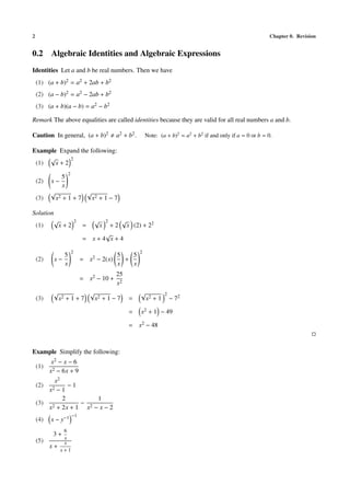
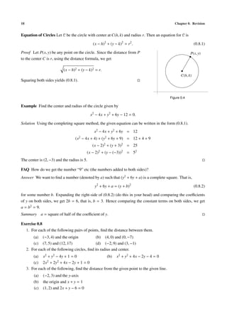
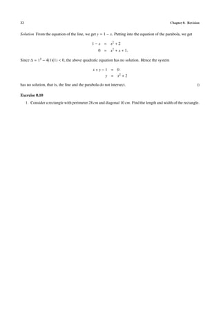
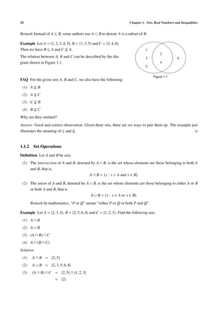
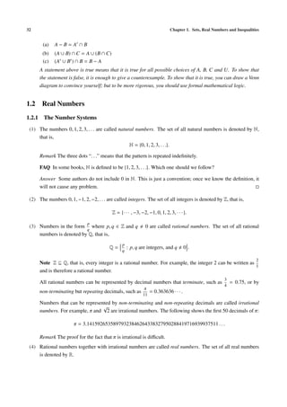
Real Number Line Real numbers can be represented by points on a line, called the real number line.
| | | | >
−1 0 1 2
Figure 1.4
Notation The following nine types of subsets of R are called intervals:
[a, b] = {x ∈ R : a ≤ x ≤ b} (1.2.1)
(a, b) = {x ∈ R : a < x < b} (1.2.2)
[a, b) = {x ∈ R : a ≤ x < b} (1.2.3)
(a, b] = {x ∈ R : a < x ≤ b} (1.2.4)
[a, ∞) = {x ∈ R : a ≤ x} (1.2.5)
(a, ∞) = {x ∈ R : a < x} (1.2.6)
(−∞, b] = {x ∈ R : x ≤ b} (1.2.7)
(−∞, b) = {x ∈ R : x < b} (1.2.8)
(−∞, ∞) = R (1.2.9)
where a and b are real numbers with a < b and ∞ and −∞ (read “infinity” and “minus infinity”) are just symbols
but not real numbers.
FAQ What are the meaning of ∞ and −∞?
Answer Intuitively, you may imagine that there is a point, denoted by ∞, very far away on the right (and −∞
on the left). So (a, ∞) is the set whose elements are the points between a and ∞, that is, real numbers greater
than a.
Remark The notation (a, b), where a < b, has two different meanings. It denotes an ordered pair as well as an
interval. To avoid ambiguity, some authors use ]a, b[ to denote the open interval {x ∈ R : a < x < b}. In this
course, we will not use this notation. Readers can determine the meaning from the context.
Terminology
• Intervals in the form (a, b), [a, b], (a, b] and [a, b) are called bounded intervals and those in the form
(−∞, b), (−∞, b], (a, ∞), [a, ∞) and (−∞, ∞) are called unbounded intervals.
• Intervals in the form (a, b), (−∞, b), (a, ∞) and (−∞, ∞) are called open intervals. For each of such
intervals, the endpoint(s), if there is any, does not belong to the interval.
• Intervals in the form [a, b], (−∞, b], [a, ∞) and (−∞, ∞) are called closed intervals. For each of such
intervals, the endpoint(s), if there is any, belongs to the interval.
• Intervals in the form [a, b] are called closed and bounded intervals.](https://image.slidesharecdn.com/basiccalculus-120628005326-phpapp02/85/Basic-calculus-41-320.jpg)
![34 Chapter 1. Sets, Real Numbers and Inequalities
• A set {a} with exactly one element of R is called a degenerated interval (its length is 0).
• Some authors also include ∅ as an interval (called the empty interval).
In this course, an interval means a nonempty, non-degenerated interval, that is, an infinite subset of R that can
be written in the form (1.2.1), (1.2.2), (1.2.3), (1.2.4), (1.2.5), (1.2.6), (1.2.7), (1.2.8) or (1.2.9).
Example For each of the following pairs of intervals A and B,
(1) A = [1, 5] and B = (3, 10]
(2) A = [−2, 3] and B = (7, 11]
(3) A = [−7, −2) and B = [−2, ∞)
• determine whether it is (i) an open interval, (ii) a closed interval , (iii) a bounded interval;
• find A ∩ B and determine whether it is an interval.
• find A ∪ B and determine whether it is an interval.
Solution
(1) Both A and B are not open intervals.
A is a closed interval but B is not a closed interval.
Both A and B are bounded intervals.
A ∩ B = (3, 5]; it is an interval.
A ∪ B = [1, 10]; it is an interval.
(2) Both A and B are not open intervals.
A is a closed interval but B is not a closed interval.
Both A and B are bounded intervals.
A ∩ B = ∅; it is not an interval.
A ∪ B = [−2, 3] ∪ (7, 11]; it is not an interval.
(3) Both A and B are not open intervals.
B is a closed interval but A is not a closed interval.
A is a bounded interval but B is not a bounded interval.
A ∩ B = ∅; it is not an interval.
A ∪ B = [−7, ∞); it is an interval.
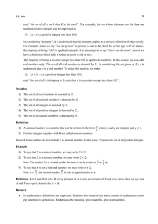
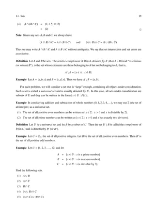
1.2.2 Radicals
Definition
(1) Let a and b be real numbers and let q be a positive integer. If aq = b, we say that a is a qth root of b.
Example
(a) −2 is the cube root of −8.
(b) 3 and −3 are the square roots of 9.](https://image.slidesharecdn.com/basiccalculus-120628005326-phpapp02/85/Basic-calculus-42-320.jpg)
![36 Chapter 1. Sets, Real Numbers and Inequalities
(3) Let b be a positive real number. Let p and q be integers where q > 0. We define
p √
q
bq = bp,
√
q p
which is the same as b .
2 √
3 √
3
Example 8 3 = 82 = 64 = 4
2 √
3 2
Remark Equivalently, we have 8 3 = 8 = 22 = 4.
FAQ Are the rules for exponents on page 1 valid if m and n are rational numbers?
Answer The rules remain valid for rational exponents, provided that the base is positive (this is required in the
p
definition of b q ). For example, we have b s bt = b s+t , where b > 0 and s, t ∈ Q.
m p
Proof Write s = and t = where m, n, p, q are integers with q, n > 0. Note that
n q
mq np mq + np
s= , t= and s+t = .
nq nq nq
By definition (equivalent form), we have
√
nq mq √
nq np
bs = b and bt = b .
√
nq
Denote α = b. Then we have
b s · bt = αmq · αnp
= αmq+np
= αnq(s+t)
s+t
= αnq
= b s+t
FAQ Can we define b raising to an irrational power? For example, can we define 2π ? How?
Answer This is deep question. The idea will be discussed Chapter 8.
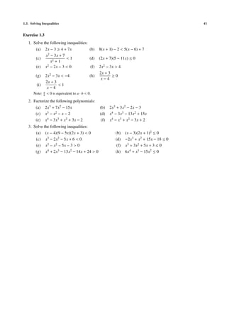
Exercise 1.2
1. Find the following sets.
(a) {x ∈ R : x2 = 2}
(b) {x ∈ R : x ≥ 0 and x2 = 2}
(c) {x ∈ Q : x2 = 2}
2. Let A = [1, 5], B = [3, 9), C = {1, 5} and D = [5, ∞). Find
(a) A ∩ B (b) A ∪ B
(c) A − C (d) B ∩ C
(e) C − B (f) B − C
(g) B − (B − C) (h) A ∪ D
(i) C ∩ D](https://image.slidesharecdn.com/basiccalculus-120628005326-phpapp02/85/Basic-calculus-44-320.jpg)
![1.3. Solving Inequalities 37
1.3 Solving Inequalities
An inequality in one unknown x can be written in one of the following forms:
(1) F(x) > 0
(2) F(x) ≥ 0
(3) F(x) < 0
(4) F(x) ≤ 0
where F is a function from a subset of R into R.
Definition Consider an inequality in the form F(x) > 0 (the other cases can be treated similarly).
(1) A real number x0 satisfying F(x0 ) > 0 is called a solution to the inequality.
(2) The set of all solutions to the inequality is called the solution set to the inequality.
To solve an inequality means to find all the solutions to the inequality, or equivalently, to find the solution set.
In this section, we consider polynomial inequalities
an xn + an−1 xn−1 + · · · + a1 x + a0 < 0 (or > 0, or ≤ 0, or ≥ 0) (1.3.1)
where n ≥ 1 and an 0.
When n = 1, (1.3.1) is a linear inequality. A revision for solving linear inequalities is given in Chapter 0.
In the following examples, we consider several linear inequalities simultaneously.
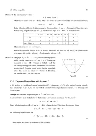
Example Find the solution set to the following compound inequality:
1 ≤ 3 − 2x ≤ 9
Solution The inequality means
1 ≤ 3 − 2x and 3 − 2x ≤ 9.
Solving them separately, we get
2x ≤ 2 −6 ≤ x
and
x ≤ 1 −3 ≤ x.
The solution set is {x ∈ R : x ≤ 1 and − 3 ≤ x} = {x ∈ R : −3 ≤ x ≤ 1}.
Remark Using interval notation, the solution set can be written as [−3, 1].
Example Find the solution set to the following:
2x + 1 < 3 and 3x + 10 < 4.
Give your answer using interval notation.
Solution Solving the inequalities separately, we get
2x < 2 3x < −6
and
x < 1 x < −2.](https://image.slidesharecdn.com/basiccalculus-120628005326-phpapp02/85/Basic-calculus-45-320.jpg)
![40 Chapter 1. Sets, Real Numbers and Inequalities
Theorem 1.3.1 Let
p(x) = cn xn + cn−1 xn−1 + · · · + c1 x + c0
be a polynomial of degree n where c0 , c1 , . . . , cn ∈ Z. Suppose (ax − b) is a factor of p(x) where a, b ∈ Z. Then
a divides cn and b divides c0 .
FAQ Can we use Factor Theorem to find all the linear factors?
Answer If some linear factors are repeated more than once, we can’t determine which one is repeated (and also
how many times?). For example, let p(x) = x3 − 3x + 2. Using Factor Theorem, we get linear factors (x − 1)
and (x + 2). It is incorrect to write p(x) = (x − 1)(x + 2). Indeed, we have
p(x) = (x − 1)2 (x + 2).
Remark We say that (x − 1) is a factor of p(x) repeated twice.
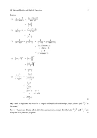
Example Find the solution set to the inequality x3 + 3x2 − 4x − 12 ≤ 0.
Solution Factorizing the polynomial p(x) on the left side we obtain
p(x) = x3 + 3x2 − 4x − 12 = (x − 2)(x + 2)(x + 3).
The sign of p(x) can be determined from the following table:
x < −3 x = −3 −3 < x < −2 x = −2 −2 < x < 2 x=2 2<x
x−2 − − − − − 0 +
x+2 − − − 0 + + +
x+3 − 0 + + + + +
p(x) − 0 + 0 − 0 +
The solution set is {x ∈ R : x ≤ −3 or − 2 ≤ x ≤ 2} = (−∞, −3] ∪ [−2, 2].
FAQ Can we use Method 1 described in Section 1.3.1?
Answer You can use that method. However the “and/or” logic is more complicated. If the degree of the
polynomial is 3, there are 4 cases; if the degree is 4, there are 8 cases. The number of cases doubles if the
degree increases by 1.
For the table method, if the degree increases by 1, the number of factors and the number of intervals increase
by (at most) 1 only.
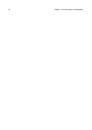
FAQ Can we use graphical method?
Answer If you know the graph of y = x3 + 3x2 − 4x − 12, y = x3 + 3x2 − 4x − 12
10
you can write down the solution immediately. For that,
5
you need to know the x-intercepts (obtained by factoring
the polynomial) and also the shape of the graph (on which -4 -3 -2 -1 1 2
-5
interval is the graph going up or down?). This will be dis-
-10
cussed in Chapter 5.
Figure 1.6](https://image.slidesharecdn.com/basiccalculus-120628005326-phpapp02/85/Basic-calculus-48-320.jpg)
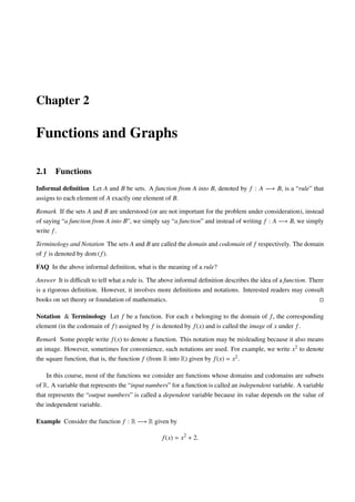
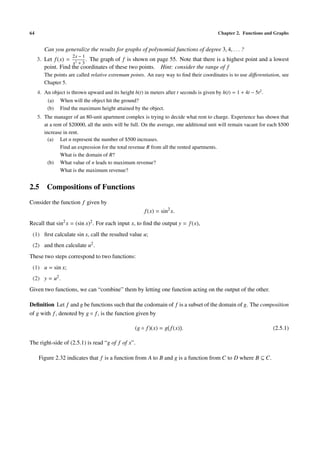
![44 Chapter 2. Functions and Graphs
We may also write y = x2 + 2 to represent this function. For each input x, the function gives exactly one output
x2 + 2, which is y. If x = 3, then y = 11; if x = 6, then y = 38 etc. The independent variable is x and the
dependent variable is y.
Example Let g(x) = x2 − 3x + 7. Find the following:
(1) g(10)
(2) g(a + 1)
(3) g(r2 )
(4) g(x + h)
g(x + h) − g(x)
(5)
h
Solution
(1) g(10) = 102 − 3(10) + 7
= 77
(2) g(a + 1) = (a + 1)2 − 3(a + 1) + 7
= (a2 + 2a + 1) − 3a − 3 + 7
= a2 − a + 5
(3) g(r2 ) = (r2 )2 − 3(r2 ) + 7
= r4 − 3r2 + 7
(4) g(x + h) = (x + h)2 − 3(x + h) + 7
= x2 + 2xh + h2 − 3x − 3h + 7
g(x + h) − g(x) [(x + h)2 − 3(x + h) + 7] − (x2 − 3x + 7)
(5) =
h h
(x 2 + 2xh + h2 − 3x − 3h + 7) − (x2 − 3x + 7)
=
h
2xh + h 2 − 3h
=
h
= 2x + h − 3
Exercise 2.1
x−5
1. Let f (x) = . Find the following:
x2 + 4
(a) f (2) (b) f (3.5)
√
(c) f (a + 1) (d) f ( a)
(e) f (a2 ) (f) f (a) + f (1)
x √
2. Let f (x) = and g(x) = x − 1. Find the following:
x+1
(a) f (1) + g(1) (b) f (2)g(2)
f (3)
(c) (d) f (a − 1) + g(a + 1)
g(3)
(e) f (a2 + 1)g(a2 + 1)](https://image.slidesharecdn.com/basiccalculus-120628005326-phpapp02/85/Basic-calculus-52-320.jpg)
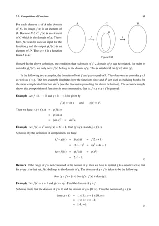
![46 Chapter 2. Functions and Graphs
Definition Let f : A −→ B be a function and let S ⊆ A. The image of S under f , denoted by f [S ], is the
subset of B given by
f [S ] = {y ∈ B : y = f (x) for some x ∈ S }.
Note f [S ] is the subset of B consisting of all the images under f of elements in S .
Example
(1) Let f : R −→ R be the function given by f (x) = x2 . For S = {1, 2, 3}, we have f [S ] = {1, 4, 9}.
(2) Let f : R −→ R be the function given by f (x) = 2x + 1. For S = [0, 1], we have f [S ] = [1, 3].
Definition Let f : A −→ B be a function. The range of f , denoted by ran ( f ), is the image of A under f , that
is, ran ( f ) = f [A].
Remark By definition, ran ( f ) = {y ∈ B : y = f (x) for some x ∈ A}. The condition
(∗) y = f (x) for some x ∈ A
means that y is an output (image) corresponding to some input (element of A). When A and B are subsets of R,
(∗) means that the equation
y = f (x)
has at least one solution belonging to A.
Example Let f : R −→ R be the function given by f (x) = x2 + 2. Then
(1) 3 belongs to the range of f because f (1) = 3, that is, 3 is the image of 1 under f . In terms of solving
equation, 3 belongs to the range means that the equation 3 = x2 + 1 has solution in R (the domain of f ).
Indeed, the equation has two solutions in R, namely 1 and −1;
(2) 2 belongs to the range because the equation 2 = x2 + 2 has solution in R, namely, 0;
(3) 1 does not belong to the range because the equation 1 = x2 + 2 has no solution in R.
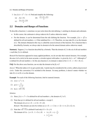
Steps to find range of function To find the range of a function f described by formula, where the domain is
taken to be the natural domain:
(1) Put y = f (x).
(2) Solve x in terms of y.
(3) The range of f is the set of all real numbers y such that x can be solved.
Example For each of the following functions, find its range.
(1) f (x) = x2 + 2
1
(2) g(x) =
x−2
√
(3) h(x) = 1 + 5x
Solution
(1) Put y = f (x) = x2 + 2.](https://image.slidesharecdn.com/basiccalculus-120628005326-phpapp02/85/Basic-calculus-54-320.jpg)
![48 Chapter 2. Functions and Graphs
• x2 + 2x − 15 ≥ 0
(x + 5)(x − 3) ≥ 0 x < −5 x = −5 −5 < x < 3 x=3 x>3
x−3 − − − 0 +
x+5 − 0 + + +
(x − 3)(x + 5) + 0 − 0 +
thus, x ≤ −5 or x ≥ 3.
Therefore, we have dom ( f ) = {x ∈ R : x ≥ −7 and (x ≤ −5 or x ≥ 3)}
= {x ∈ R : (x ≥ −7 and x ≤ −5) or (x ≥ −7 and x ≥ 3)}
= {x ∈ R : −7 ≤ x ≤ −5 or x ≥ 3}
= [−7, −5] ∪ [3, ∞).
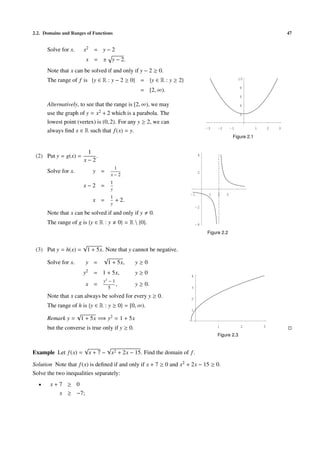
2x + 1
Example Let f (x) = . Find the range of f .
x2 + 1
Solution
2x + 1
Put y = f (x) = 2 .
x +1
2x + 1
Solve for x. y =
x2 + 1
yx2 + y = 2x + 1
yx2 − 2x + (y − 1) = 0
2 ± 4 − 4y(y − 1) −1
x = if y 0, x = if y = 0,
2y 2
1 ± 1 − y2 + y
= if y 0.
y
Combining the two cases, we see that x can be solved if and only if 1 − y2 + y ≥ 0, that is, y2 − y − 1 ≤ 0.
The range of f is {y ∈ R : y2 − y − 1 ≤ 0}.
√
1± 5
y2
To solve the inequality − y − 1 ≤ 0, first we find the zero of the left-side by quadratic formula to get .
√ √ 2
1− 5 1+ 5
By the factor theorem and comparing coefficient of y2 , we see that y2 − y − 1 = y − y−
2 2
√ √ √ √ √ √
1− 5 1− 5 1− 5 1+ 5 1+ 5 1+ 5
y< 2 y= 2 2 <y< 2 y= 2 y> 2
√
1− 5
y− 2 − 0 + + +
√
1+ 5
y− 2 − − − 0 +
y2 − y − 1 + 0 − 0 +
√ √
1− 5 1+ 5
From the table, we see that ran ( f ) = y∈R: ≤y≤
2 2
√ √
1− 5 1+ 5
= ,
2 2](https://image.slidesharecdn.com/basiccalculus-120628005326-phpapp02/85/Basic-calculus-56-320.jpg)
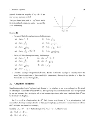
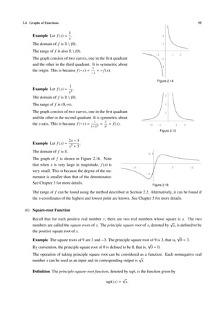
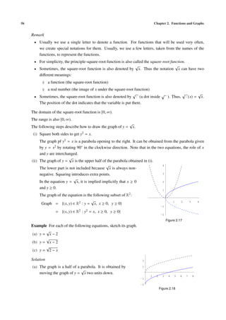
![2.4. Graphs of Functions 53
2.4 Graphs of Functions
Let f : A −→ R be a function where A ⊆ R. The graph of f is the following subset of R2 :
(x, y) ∈ R2 : x ∈ A and y = f (x) .
Example
(1) Constant Functions A constant function is a function f that is given by
f (x) = c,
where c is a constant (a real number).
The domain of every constant function is R.
c
The range is a singleton: {c}.
The graph is a horizontal line whose y-intercept
is (0, c).
Figure 2.10
Remark Let f (x) = x0 . Note that for all x 0, we have f (x) = 1 and that f (0) is undefined. So there is
a small difference between f and the constant function 1 whose domain is R. However, for convenience,
we treat the function x0 as the constant function 1.
In the above discussion, we use the symbol 1 to represent the function with domain and codomain equal
to R and assigning every x ∈ R to the number 1. Thus the symbol 1 has two different meanings. It may be
a function or a number. This abuse of notation is sometimes used in mathematics. Readers can determine
the meaning from the context.
(2) Linear Functions A linear function is a function f given by
f (x) = ax + b,
where a and b are constants and a 0.
The domain of every linear function is R.
b
The range is also R (note that a is assumed to be non-zero).
The graph is a line with slope a and y-intercept (0, b).
Figure 2.11
(3) Quadratic Functions A quadratic function is a function f given by
f (x) = ax2 + bx + c,
where a, b and c are constants and a 0.
The domain of every quadratic function is R.
The range is [k, ∞) if a > 0 and (−∞, k] if a < 0 where k is the y-coordinate of the vertex.
The graph is a parabola which opens upward if a > 0 and downward if a < 0.](https://image.slidesharecdn.com/basiccalculus-120628005326-phpapp02/85/Basic-calculus-61-320.jpg)
![54 Chapter 2. Functions and Graphs
a>0
a<0
Figure 2.12(a) Figure 2.12(b)
Remark Besides using the completing square method to find the vertex, we can also use differentiation
(see Chapter 5).
(4) Polynomial Functions A function f given by
f (x) = an xn + an−1 xn−1 + · · · + a1 x + a0 ,
where a0 , a1 , . . . , an are constants with an 0, is called a polynomial function of degree n.
If n = 0, f is a constant function.
If n = 1, f is a linear function.
If n = 2, f is a quadratic function.
2
Example Let f (x) = x3 − 3x2 + x − 1.
1 2
The graph of f is shown in Figure 2.13.
-1
-2
In Chapter 5, we will discuss how to sketch graphs of poly-
-4
nomial functions.
-6
Figure 2.13
The domain of every polynomial function f is R.
There are three possibilities for the range.
(a) If the degree is odd, then ran ( f ) = R.
(b) If the degree is even and positive, then
(i) ran ( f ) = [k, ∞) if an > 0;
(ii) ran ( f ) = (−∞, k] if an < 0,
where k is the y-coordinate of the lowest point for case (i), or the highest point for case (ii), of the
graph.
Remark The constant function 0 is also considered to be a polynomial function. However, its degree is
assigned to be −∞ (for convenience of a rule for degree of product of polynomials).
(5) Rational Functions A rational function is a function f in the form
p(x)
f (x) = ,
q(x)
where p and q are polynomial functions.](https://image.slidesharecdn.com/basiccalculus-120628005326-phpapp02/85/Basic-calculus-62-320.jpg)
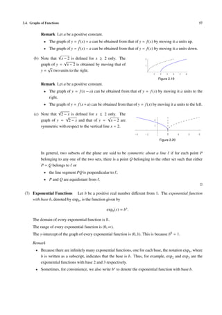
![2.4. Graphs of Functions 59
For simplicity, we write sin(x) = sin x etc.
• The sine function: sin
The domain of the sine function is R.
The range is [−1, 1].
The graph of the sine function has a waveform as shown in Figure 2.24 (the symbol p stands for the
number π). The graph is symmetric about the origin. This is because sin(−x) = − sin x. The graph
crosses the x-axis infinitely often, at points with x-coordinates 0, ±π, ±2π, . . .
1
-4p -2p 2p 4p
-1
Figure 2.24
The sine function is periodic with period 2π, that is, sin(x + 2π) = sin x for all x ∈ R.
Definition If f is a function such that f (x + p) = f (x) for all x ∈ dom ( f ), where p is a positive
constant, then we say that f is periodic with period p.
• The cosine function: cos
The domain of the cosine function is R.
The range is [−1, 1].
The graph of the cosine function has a waveform. It is symmetric about the y-axis. This is be-
cause cos(−x) = cos x. The graph crosses the x-axis infinitely often, at points with x-coordinates
π 3π
± ,± ,...
2 2
1
-4p -2p 2p 4p
-1
Figure 2.25
The cosine function is periodic with period 2π, that is, cos(x + 2π) = cos x for all x ∈ R.
Remark The graph of the cosine function can be obtained by shifting the graph of the sine function
π π
units to the left. This is because cos x = sin x + for all x ∈ R.
2 2](https://image.slidesharecdn.com/basiccalculus-120628005326-phpapp02/85/Basic-calculus-67-320.jpg)
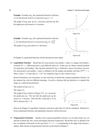
![2.4. Graphs of Functions 61
(d) |a − b| is the distance between a and b.
√
(e) a2 = |a|.
The domain of | · | is R.
The range is [0, ∞).
The graph of the absolute value function a V-shape figure.
It is the union of the following three subsets of R2 . 2
• {(x, y) ∈ R2 : x > 0 and y = x} which is the half-
1
line in the first quadrant with slope equal to 1, starting
from the origin but not including the origin.
• {(x, y) ∈ R2 : x = 0 and y = 0} which is the point -2 -1 1 2
{0, 0}, that is, the origin.
-1
• {(x, y) ∈ R2 : x < 0 and y = −x} which is the half-line
in the second quadrant with slope equal to −1, starting -2
from the origin but not including the origin. Figure 2.27
Remark We may also define the absolute value function in the following ways:
x if x ≥ 0,
(i) |x| =
−x if x < 0.
x if x > 0,
(ii) |x| =
−x if x ≤ 0.
x if x ≥ 0,
(iii) |x| =
−x if x ≤ 0.
In (i) or (ii), the domain R is divided into two disjoint subsets.
In (iii), although R is the union of (−∞, 0] and [0, ∞), the two subsets are not disjoint; the number 0
belongs to both. However, this will not cause any problem to define |0| because if we use the first rule,
we get |0| = 0 and if we use the second rule, we get |0| = −0 = 0. We say that |0| is well-defined because
its value does not depend on the choice of the rule.
Example For each of the following equations, sketch its graph.
(a) y = 1 − |x|
(b) y = |x − 1|
Solution
(a) By the definition of the absolute value function, the equation is
1−x
if x > 0,
y= 1−0
if x = 0,
1 − (−x) if x < 0.
The graph is shown in Figure 2.28. It consists of the half-line y = 1 − x, x > 0, the point (0, 1) and
the half-line y = 1 + x, x < 0.](https://image.slidesharecdn.com/basiccalculus-120628005326-phpapp02/85/Basic-calculus-69-320.jpg)
![62 Chapter 2. Functions and Graphs
Remark Alternatively, the graph can be obtained as 1
follows:
• The graph of y = −|x| and that of y = |x| are
1 2
symmetric about the x-axis. So the graph of
-2 -1
y = −|x| is an inverted V-shape figure. -1
• Move the inverted V-shape figure 1 unit up.
-2
Figure 2.28
(b) The graph of y = |x − 1| is a V-shape figure. It can
2
be obtained by moving the graph of y = |x| one unit
to the right. 1
-2 -1 1 2 3
Figure 2.29
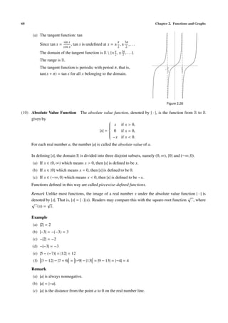
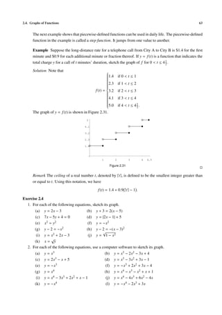
(11) Piecewise-defined Functions Below we give more examples of piecewise-defined functions.
Example Let f : [−2, 6] −→ R be the function given by
x2
if − 2 ≤ x < 0
f (x) = 2x if 0 ≤ x < 2
4 − x if 2 ≤ x ≤ 6.
For each of the following, find its value:
(a) f (−1)
1
(b) f
2
(c) f (3)
Sketch the graph of f .
Solution
(a) f (−1) = (−1)2 = 1
1 1
(b) f =2· =1
2 2
(c) f (3) = 4 − 3 = 1 4
The graph of f consists of three parts:
• the curve y = x2 , −2 ≤ x < 0 (part of a parabola); 2
• the line segment y = 2x, 0 ≤ x < 2 (excluding the
right endpoint);
• the line segment y = 4 − x, 2 ≤ x ≤ 6. -2 2 4 6
-2
Figure 2.30
Remark In the figure, the little circle indicates that the point (2, 4) is not included in the graph. The little
dot (which can be omitted) emphasizes that the point (2, 2) is included.](https://image.slidesharecdn.com/basiccalculus-120628005326-phpapp02/85/Basic-calculus-70-320.jpg)
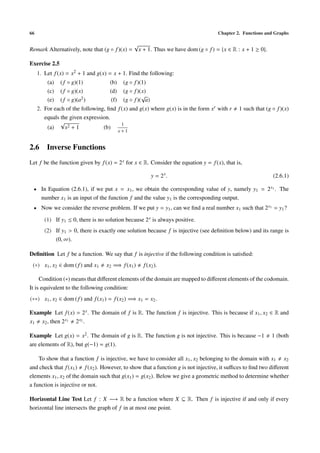
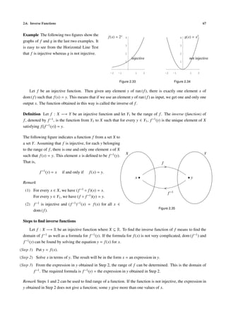
![68 Chapter 2. Functions and Graphs
Example Let f (x) = 2x3 + 1. Find the inverse of f .
Solution The domain of f is R. It is not difficult to show that f is injective and that the range of f is R. These
two facts can also be seen from the following steps:
Put y = f (x). That is, y = 2x3 + 1.
Solve for x: y − 1 = 2x3
y−1
= x3
2
3 y−1
= x (x can be solved for all real numbers y)
2
3 y−1
Thus we have dom ( f −1 ) = R and f −1 (y) = .
2
Example Let g : [0, ∞) −→ R be the function given by g(x) = x2 . Find the inverse of g.
Solution Because the domain of g is [0, ∞), the function g is injective . Moreover, the range of g is [0, ∞).
These two facts can also be seen from the following steps:
Put y = g(x). That is, y = x2 . Note that y ≥ 0 and that x ≥ 0 since x ∈ dom ( f ).
Solve for x: y = x2 , y ≥ 0, x ≥ 0
√ √
y = x (x can be solved if and only if y ≥ 0, x = − y is rejected)
√
Thus we have dom (g−1 ) = [0, ∞) and g−1 (y) = y.
Remark Usually, we use x to denote the independent variable of a function. For the above examples, we may
x−1 √
write f −1 (x) = 3 and g−1 (x) = x.
2
1
Caution f −1 (x)
f (x)
Remark We use sin−1 or arcsin to denote the inverse of sin etc. 1
y = sin x
Although the sine function is not injective, we can make it injec-
tive by restricting the domain to [− π , π ].
2 2
p p
x = sin−1 y means sin x = y and − π ≤ x ≤
2
π
2. The domain of -
2 2
sin−1 is [−1, 1] because −1 ≤ sin x ≤ 1.
-1
Figure 2.36
FAQ Why do we use the notation f −1 ?
Answer The following example gives a reason why we use such a notation. Let f (x) = 2x. Then f is injective
1 1
and its inverse is given by f −1 (x) = x. The multiplicative constant is 2−1 .
2 2
Another reason is to have the “index law” (details omitted):
f m ◦ f n = f m+n for m, n ∈ Z.](https://image.slidesharecdn.com/basiccalculus-120628005326-phpapp02/85/Basic-calculus-76-320.jpg)
![Chapter 3
Limits
Calculus is the study of differentiation and integration (this is indicated by the Chinese translation of “calcu-
lus”). Both concepts of differentiation and integration are based on the idea of limit. In this chapter, we use an
intuitive approach to consider limits, omitting the more difficult -δ definition.
3.1 Introduction
In this section, we introduce the idea of limit by considering two problems. The first problem is to “find” the
velocity of an object at a particular instant. The idea is related to differentiation. The second problem is to
“find” the area under the graph of a curve (and above the x-axis). The idea is related to integration.
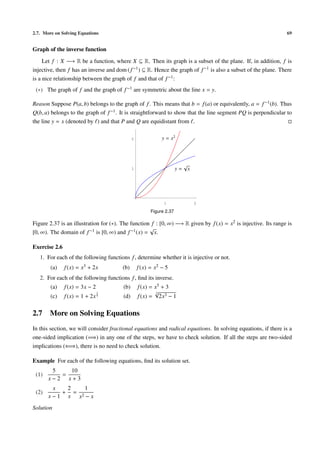
Problem 1 Suppose an object moves along the x-axis and its displacement (in meters) s at time t (in seconds)
is given by
s(t) = t2 , t ≥ 0.
We want to consider its velocity at a certain time instant, say at t = 2.
Idea Velocity (or speed) is defined by
distance traveled
velocity = (3.1.1) distance
time elapsed
(3.1.1) can only be applied to find average velocities over time intervals. time
We (still) don’t have a definition for velocity at t = 2.
Figure 3.1
To define the velocity at t = 2, we consider short time intervals
1
about t = 2, say from t = 2 to t = 2 + n . Using (3.1.1), we n Time interval Velocity
2
can compute the average velocity over the time intervals [2, 2.5], 1 [2,2.5] 4.5 m/s
[2, 2.25] etc. 2 [2,2.25] 4.25 m/s
3 [2,2.125] 4.125 m/s
4 [2,2.0625] 4.0625 m/s
.
.
.](https://image.slidesharecdn.com/basiccalculus-120628005326-phpapp02/85/Basic-calculus-81-320.jpg)
![74 Chapter 3. Limits
1
In general, the velocity vn over the time interval 2, 2 + is
2n
1 2
(2 + 2n ) − 22
vn = 1
2n
1 1 2
4+2·2· 2n + 2n −4 1
= = 4+ .
1
2n
2n
It is clear that if n is very large (that is, if the time interval is very short), vn is very close to 4. The velocity,
called the instantaneous velocity, at t = 2 is (defined to be) 4.
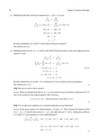
Problem 2 Find the area of the region that lies under the curve y = x2 and
1
above the x-axis for x between 0 and 1.
1
Figure 3.2
Idea Similar to the idea in Problem 1, we use approximation to find/define
area. First we divide the interval [0, 1] into finitely many subintervals of equal
lengths: 1
1 1 2 2 3 n−1
0, , , , , , ..., ,1 .
n n n n n n
i−1 i
For each subinterval , , we consider the rectangular region with base on
n n
i−1 2
the subinterval and height (the largest region that lies under the curve).
n
If we add the area of these rectangular regions, the sum is smaller than that of
the required region. However, if n is very large, the error is very small and we
get a good approximation for the required area. 1
Figure 3.3
The following table gives the sum S n of the areas of the rectangular regions (correct
to 3 decimal places) for several values of n.
In general, if there are n subintervals, the sum S n is
n Sum of areas
2 2 2
1 2 1 1 1 2 1 n−1 2 0.125
Sn = ·0 + · + · + ··· + ·
n n n n n n n 3 0.185
12 + 22 + · · · + (n − 1)2 4 0.219
= .
n3 .
.
n(n − 1)(2n − 1) 10 0.285
= By Sum of Squares Formula
6n3 .
.
.
2n3 − 3n2 + n 100 0.328
=
6n3 .
.
.
1 1 1
= − + 2 500 0.332
3 2n 6n
1
It is clear that if n is very large (so that the error is small), S n is very close to .
3](https://image.slidesharecdn.com/basiccalculus-120628005326-phpapp02/85/Basic-calculus-82-320.jpg)
![3.2. Limits of Sequences 75
1
Conclusion The area of the region is .
3
n(n + 1)(2n + 1)
Sum of Squares Formula 12 + 22 + · · · + n2 =
6
Exercise 3.1
∗ 1. 1
In the first problem: If we consider short time intervals other than 2, 2 + , for example consider
2n
1 1
2, 2 + or 2 − n2
,2 , do we get the same result?
n
∗ 2. In the second problem:
(a) For each subinterval, we use the value of y at the left endpoint as the height of the rectangular
region. If we take the right endpoint instead (we will get a surplus in this case), do we get the
same result? How about taking an arbitrary point in each subinterval?
(b) In finding the approximations, we divide [0, 1] into equal subintervals. How about dividing it into
unequal subintervals?
3.2 Limits of Sequences
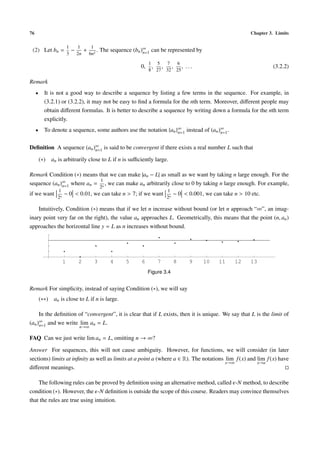
In the last section, we obtained formulas for vn and S n in Problems 1 and 2 respectively. Each of these formulas
gives a sequence (which is a special type of function). To consider the behavior of a sequence for large n, we
introduce the concept of limit of a sequence.
Definition
• A sequence is a function whose domain is Z+ (the set of all positive integers).
• A sequence of real numbers is a sequence whose codomain is R.
A sequence of real numbers is a function from Z+ to R. In this course, we will not consider sequences with
codomains different from R. Thus, in what follows, a sequence means a sequence of real numbers.
Let f : Z+ −→ R be a sequence. For each positive integer n, the value f (n) is called the nth term of the
sequence and is usually denoted by a small letter together with n in the subscript, for example an . The sequence
is also denoted by (an )∞ because if we know all the an ’s, then we know the sequence.
n=1
Sometimes, we represent a sequence (an )∞ by listing a few terms in the sequence:
n=1
a1 , a2 , a3 , a4 , a5 , . . .
In the following example, the sequences (an )∞ and (bn )∞ are the sequences obtained in Problem 1 and
n=1 n=1
Problem 2 in the last section respectively.
Example
1
(1) Let an = 4 + . The sequence (an )∞ can be represented by
n=1
2n
9 17 33 65
, , , , ... (3.2.1)
2 4 8 16](https://image.slidesharecdn.com/basiccalculus-120628005326-phpapp02/85/Basic-calculus-83-320.jpg)
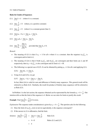
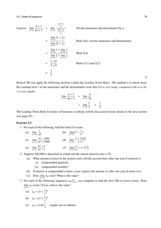
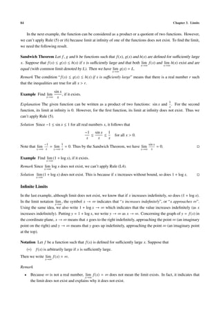
![3.3. Limits of Functions at Infinity 81
The following rules for limits of functions at infinity are similar to that for limits of sequences. In (4), (5),
(5s) and (6), f and g are functions such that f (x) and g(x) are defined for sufficiently large x.
Rules for Limits of Functions at Infinity
(L1) lim k = k (where k is a constant)
x→∞
1
(L2) lim = 0 (where p is a positive constant)
x→∞ xp
1
(L3) lim =0 (where b is a constant greater than 1)
x→∞ bx
(L4) lim f (x) ± g(x) = lim f (x) ± lim g(x)
x→∞ x→∞ x→∞
The result is valid for sum and difference of finitely many functions.
(L5) lim f (x) · g(x) = lim f (x) · lim g(x)
x→∞ x→∞ x→∞
The result is valid for product of finitely many functions.
(L5s) lim k · g(x) = k · lim g(x)
x→∞ x→∞
f (x) x→∞ f (x)
lim
(L6) lim = provided that lim g(x) 0.
x→∞ g(x) lim g(x) x→∞
x→∞
To consider limits of functions at infinity, we should first check the domains of the functions. For example,
√
if f (x) = 1 − x, the domain of f is {x ∈ R : 1 − x ≥ 0} = (−∞, 1]; it is meaningless to talk about limit of f at
2
infinity. In the next example, the domain of the function 1 − 3 is R {0}; the function is defined for large x and
x
hence we may consider its limit at infinity (whether the limit exists; and if exists, find the value).
2
Example Find lim 1 − , if it exists.
x→∞ x3
2 1
Solution lim 1 − = lim 1 − lim 2 · Rule (L4), rewrite 2nd term
x→∞ x3 x→∞ x→∞ x3
1
= 1 − 2 · lim Rules (L1) and (L5s)
x→∞ x3
= 1−2·0 Rule (L2)
= 1
Example Find lim 2−x + 3 , if it exists.
x→∞
Solution lim (2−x + 3) = lim 2−x + lim 3 Rule (L4)
x→∞ x→∞ x→∞
1
= lim +3 Rewrite first term and Rule (L1)
x→∞ 2 x
= 0+3 Rule (L3)
= 3](https://image.slidesharecdn.com/basiccalculus-120628005326-phpapp02/85/Basic-calculus-89-320.jpg)
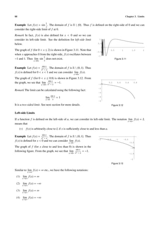
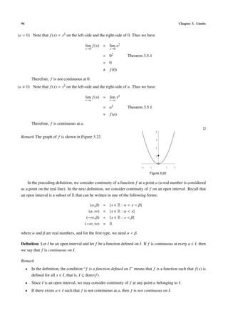
![98 Chapter 3. Limits
Explanation The result means that if f is a rational function and if I is an open interval with I ⊆ dom ( f ), then
p(x)
f is continuous on I. Recall that f can be written in the form f (x) = where p(x) and q(x) are polynomials.
q(x)
• If q(x) is never 0, then dom ( f ) = R.
• If q(x) = 0 has solutions, then dom ( f ) is the union of finitely many open intervals:
dom ( f ) = R {z1 , z2 , . . . , zk−1 , zk } = (−∞, z1 ) ∪ (z1 , z2 ) ∪ · · · ∪ (zk−1 , zk ) ∪ (zk , ∞),
where z1 , . . . , zk are the (distinct) solutions arranged in increasing order.
p(x)
Proof Let f be a rational function, that is, f (x) = where p(x) and q(x) are polynomials. Let I be an open
q(x)
interval with I ⊆ dom ( f ). For every a ∈ I, we have a ∈ dom ( f ) and so by the definition of domain, we have
p(a)
q(a) 0. Therefore, by Theorem 3.5.2, we have lim f (x) = = f (a), that is, f is continuous at a. Thus by
x→a q(a)
definition, f is continuous on I.
In the preceding definition, we consider continuity on open intervals. If the domain of a function f is in the
form [a, b), we cannot talk about continuity of f at a because f is not defined on the left-side of a. Since f is
defined on the right-side of a, we may consider lim f (x) and also whether the right-side limit equals f (a).
x→a+
Definition Let a be a real number and let f be a function defined on the right-side of a as well as at a. If
lim f (x) = f (a), then we say that f is right-continuous at a.
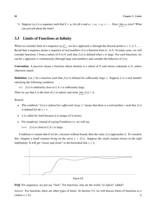
x→a+
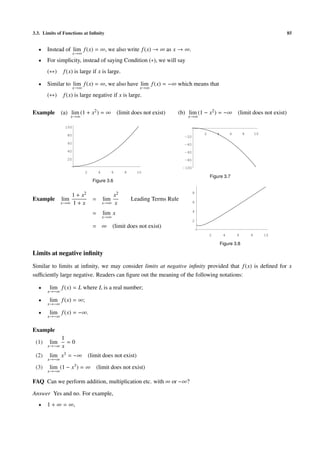
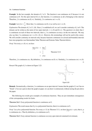
√
Example Let f (x) = x. The domain of f is [0, ∞). Using a rule
similar to Rule (La2 ), we get
2
√
lim f (x) = lim x 1.5
x→0+ x→0+
1
= 0
0.5
= f (0).
1 2 3 4
Therefore, f is right-continuous at 0.
Figure 3.24
In the above example, f is also continuous at every a > 0. Thus, it is “continuous” at every a belonging to
its domain, where “continuous at 0” means right-continuous at 0.
Definition Let I be an interval in the form [c, d) where c is a real number and d is ∞ or a real number greater
than c. Let f be a function defined on I. We say that f is continuous on I if it is continuous at every a ∈ (c, d)
and is right-continuous at c.
Similar to the above treatment, we may also consider continuity of functions f defined on intervals in the
form (c, d] or [c, d].
Definition Let a be a real number and let f be a function defined on the left-side of a as well as at a. If
lim f (x) = f (a), then we say that f is left-continuous at a.
x→a−
Definition Let I be an interval in the form (c, d] where d is a real number and c is −∞ or a real number less
than d. Let f be a function defined on I. We say that f is continuous on I if it is continuous at every a ∈ (c, d)
and is left-continuous at d.](https://image.slidesharecdn.com/basiccalculus-120628005326-phpapp02/85/Basic-calculus-106-320.jpg)
![3.6. Continuous Functions 99
Definition Let I be an interval in the form [c, d] where c and d are real numbers and c < d. Let f be a function
defined on I. We say that f is continuous on I if it is continuous at every a ∈ (c, d) and is right-continuous at c
and left-continuous at d.
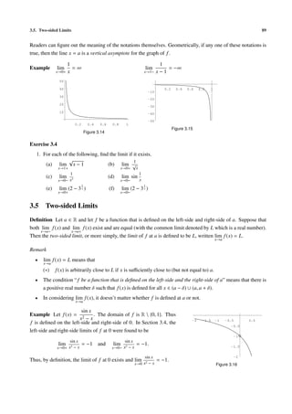
Example Let f : R −→ R be the function given by
|x| if − 1 ≤ x ≤ 1,
f (x) =
−1 otherwise.
Discuss whether f is continuous on [−1, 1].
Explanation In defining f , the word “otherwise” means that if x < −1 or x > 1; this is because it is given that
dom ( f ) = R. Thus we have f (x) = −1 if x < −1 or x > 1.
Solution It is straightforward to check that f is continuous at every a ∈ (−1, 1) and that f is left-continuous at
1 and right-continuous at −1. Thus by definition, f is continuous on [−1, 1].
Remark
• Note that f is also defined on the right-side of 1 (for example).
Thus we can also consider the continuity of f at 1. In fact, since
lim f (x) = −1 and lim f (x) = 1, it follows that lim f (x) does
x→1+ x→1− x→1
not exist and so f is not continuous at 1.
1
• Let I be an interval in the form [c, d] or [c, d) or (c, d] and let
f be a function defined on an open interval containing I. Then
1 1
for every a ∈ I, we may consider whether f is continuous at a.
The above example shows that f may be continuous on I but not 1
continuous at some a ∈ I. Figure 3.25
The following theorem describes an important property of continuous functions on intervals. The proof
requires a deep understanding of real numbers and is beyond the scope of this course.
Intermediate Value Theorem Let f be a function that is defined and continuous on an interval I . Then for
every pair of elements a and b of I , and for every real number η between f (a) and f (b), there exists a number ξ
between a and b such that f (ξ) = η.
Explanation In the theorem, the condition “ f is a function that is defined and continuous on an interval I”
means that “ f is a function, I is an interval, I ⊆ dom ( f ) and f is continuous on I”.
• Let x, y and z be real numbers. We say that z lies between x and y if
(1) x ≤ z ≤ y for the case where x ≤ y;
(2) y ≤ z ≤ x for the case where y ≤ x.
Note that if x = y, then z lies between x and y means that z = x = y.
• Because I is an interval, if a and b belong to I and a < ξ < b, then ξ belongs to I also.
• The result means that if f is a continuous function whose domain is an interval, then its range is either a
singleton (in this case, f is a constant function) or an interval.](https://image.slidesharecdn.com/basiccalculus-120628005326-phpapp02/85/Basic-calculus-107-320.jpg)
![100 Chapter 3. Limits
The following result is also called the Intermediate Value Theorem.
Corollary 3.6.3 Let f be a function that is defined and continuous on an interval I . Suppose that a and b
are elements of I such that f (a) and f (b) have opposite signs. Then there exists ξ between a and b such that
f (ξ) = 0.
Explanation The condition “ f (a) and f (b) have opposite signs” means that one of the two values is positive
and the other is negative.
Proof The result is a special case of the Intermediate Value Theorem. This is because f (a) and f (b) have
opposite signs implies that 0 lies between f (a) and f (b).
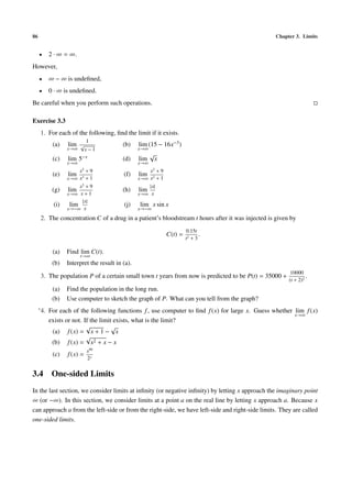
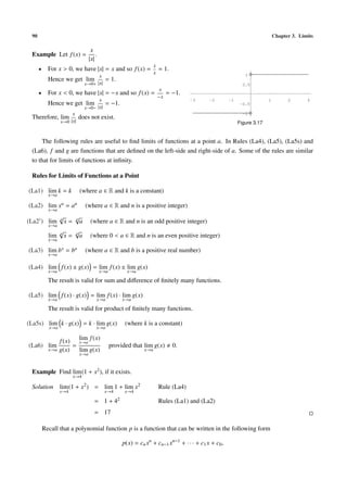
In the Intermediate Value Theorem, the assumption that f is continuous cannot be omitted. The following
example is an illustration.
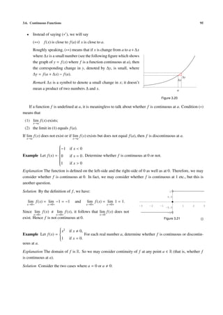
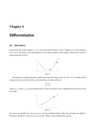
Example Let f : [0, 2] −→ R be defined by
−1 if 0 ≤ x ≤ 1,
f (x) =
1 if 1 < x ≤ 2.
1
Note that f (0) = −1 and f (2) = 1 have opposite signs. However,
0.5
there does not exist any ξ ∈ [0, 2] such that f (ξ) = 0.
We can’t apply the Intermediate Value Theorem. This is because 0.5 1 1.5 2
f is not continuous on [0, 2]. Indeed, it is not continuous at 0 -0.5
since lim f (x) and lim f (x) are not equal. -1
x→0− x→0+
Figure 3.26
Corollary 3.6.4 Let f be a function that is defined and continuous on an interval I . Suppose that f has no zero
in I . Then f is either always positive in I or always negative in I .
Explanation The condition “ f has no zero in I” means that the equation f (x) = 0 has no solution in I, that is,
f (x) 0 for all x ∈ I. The conclusion “ f is either always positive in I or always negative in I” means that
either one of the following two cases is true:
(1) f (x) > 0 for all x ∈ I;
(2) f (x) < 0 for all x ∈ I.
Proof Suppose f takes both positive and negative values in I, that is, there exist a, b ∈ I such that f (a) < 0
and f (b) > 0. Then by the Intermediate Value Theorem (Corollary 1), f has a zero between a and b which
contradicts the assumption that f has no zero in I.
The above corollary is also called the Intermediate Value Theorem. The following example illustrates how
to apply the theorem to solve inequalities.
Example Find the solution set to the inequality x3 + 3x2 − 4x − 12 ≤ 0.
Solution Let p : R −→ R be the function given by
p(x) = x3 + 3x2 − 4x − 12.](https://image.slidesharecdn.com/basiccalculus-120628005326-phpapp02/85/Basic-calculus-108-320.jpg)
![3.6. Continuous Functions 101
Factorizing we get
p(x) = (x − 2)(x + 2)(x + 3).
The zeros of the function p are −3, −2 and 2 (and no more). Since p is continuous on R, it follows from
the Intermediate Value Theorem that on each of the following intervals, p is either always positive or always
negative:
(−∞, −3), (−3, −2), (−2, 2), (2, ∞).
To determine the sign of p on each of these intervals, we can just pick a point there and find the value (sign) of
p at that point. Taking the points −4, −2.5, 0 and 3, we find that
p(−4) < 0, p(−2.5) > 0, p(0) < 0, p(3) > 0.
Thus we have
• p(x) < 0 for x < −3;
• p(x) > 0 for −3 < x < −2;
• p(x) < 0 for −2 < x < 2;
• p(x) > 0 for x > 2.
The solution set is {x ∈ R : x ≤ −3 or − 2 ≤ x ≤ 2} = (−∞, −3] ∪ [−2, 2].
Remark The above steps can be expressed in a compact form using a table:
x < −3 x = −3 −3 < x < −2 x = −2 −2 < x < 2 x=2 x>2
p(x) − 0 + 0 − 0 +
p(−4) < 0 p(−2.5) > 0 p(0) < 0 p(3) > 0
The next result describes an important property of functions continuous on closed and bounded intervals. It
has many important consequences (for example, see the proof of the Mean Value Theorem in the appendix).
Extreme Value Theorem Let f be a function that is defined and continuous on a closed and bounded interval
[a, b]. Then f attains its maximum and minimum in [a, b], that is, there exist x1 , x2 ∈ [a, b] such that
f (x1 ) ≤ f (x) ≤ f (x2 ) for all x ∈ [a, b].
Explanation The theorem is a deep result. Its proof is beyond the scope of this course and is thus omitted.
The following two examples illustrate that in the Extreme Value Theorem,
• closed intervals cannot be replaced by open intervals;
• the assumption that f is continuous cannot be omitted.](https://image.slidesharecdn.com/basiccalculus-120628005326-phpapp02/85/Basic-calculus-109-320.jpg)
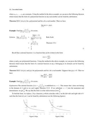
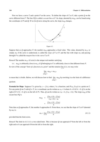
![102 Chapter 3. Limits
4
Example Let f : (0, 1) −→ R be the function given by
1 3
f (x) =
x
It is straightforward to show that f is continuous on (0, 1). However, the function f 2
does not attain its maximum nor minimum in (0, 1). This is because the range of f is
1
(1, ∞); f (x) can be arbitrarily large and it can be arbitrarily close to and greater than
1 but it can’t be equal to 1.
1
Figure 3.27
Example Let f : [0, 1] −→ R be the function given by
4
1 if x = 0,
f (x) = 1
if 0 < x ≤ 1.
3
x
The function f does not attain its maximum in [0, 1]. This is because the range of f 2
is [1, ∞); f (x) can be arbitrarily large.
1
Note that f is not right-continuous at 0 since lim f (x) = ∞ (limit does not exist).
x→0+
1
Exercise 3.6 Figure 3.28
x2
if x < 1,
1. Let f (x) = 1
if 1 ≤ x < 2,
1
if x ≥ 2.
x
(a) Sketch the graph of f for x ∈ [0, 5].
(b) Find all the point(s) in R at which f is discontinuous.
x2 + x − 2
2. Let f (x) = √ .
1− x
(a) What is the domain of f ?
(b) Find lim f (x).
x→1
(c) Can we define f (1) to make f continuous at 1? If yes, what is the value?
1
3. Let f (x) = sin .
x
(a) What is the domain of f ?
(b) Find lim f (x).
x→0
(c) Can we define f (0) to make f continuous at 0? If yes, what is the value?
4. Let p(x) = x5 − x4 − 5x3 + x2 + 8x + 4. It is given that the equation p(x) = 0 has exactly two solutions,
namely 2 and −1. Use this information to solve the inequality p(x) > 0.
5. Let p(x) = x5 − 6x4 − 3x3 + 5x2 + 7.
(a) Show that the equation p(x) = 0 has a solution between 1 and 2.
(b) It is given that p(x) = 0 has exactly one solution between 1 and 2. Is the solution closer to 1 or 2?](https://image.slidesharecdn.com/basiccalculus-120628005326-phpapp02/85/Basic-calculus-110-320.jpg)
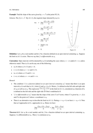
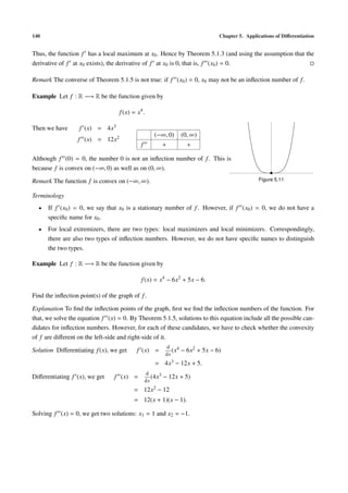
![128 Chapter 5. Applications of Differentiation
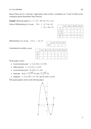
5.1 Curve Sketching
5.1.1 Increasing and Decreasing Functions
Definition Let f be a function and let I be an interval such that I ⊆ dom ( f ). We say that f is
• strictly increasing on I if for any two numbers x1 , x2 ∈ I, where x1 < x2 , we have f (x1 ) < f (x2 );
• strictly decreasing on I if for any two numbers x1 , x2 in I, where x1 < x2 , we have f (x1 ) > f (x2 ).
Remark
• In the definition, I can be an open interval, a closed interval or a half-open half-closed interval in the
form [a, b) or (a, b].
• Although we can define the concepts “ f is strictly increasing (or strictly decreasing) on a set S , where
S ⊆ dom ( f )”, we will not use such concepts in this course because the concepts “strictly increasing (or
strictly decreasing) on an interval” are good enough for our consideration; moreover, a function strictly
increasing (or strictly decreasing) on a set S 1 and also on a set S 2 may not be strictly increasing (or
strictly decreasing) on S 1 ∪ S 2 .
Geometric Meaning A function is strictly increasing (respectively strictly decreasing) on an interval I means
that for x ∈ I, the graph of f goes up (respectively goes down) as x goes from left to right.
Terminology For simplicity, instead of saying “strictly increasing”, we will say “increasing” etc.
Remark Some authors have a different definition for “increasing”. In that case, “increasing” and “strictly
increasing” refer to different concepts.
Example Let f : R −→ R be the function given by f (x) = x3 .
Then f is increasing on R.
3 3
Reason If x1 < x2 , then x1 < x2 .
Figure 5.1
1
Example Let f : (0, ∞) −→ R be the function given by f (x) = √ .
x
Then f is decreasing on (0, ∞).
√ √ 1 1
Reason If 0 < x1 < x2 , then x1 < x2 and so √ > √ .
x1 x2
Figure 5.2
Example Let f : R −→ R be the function given by f (x) = x2 .
Then f is decreasing on (−∞, 0) and increasing on (0, ∞).
Reason
• 2 2
If x1 < x2 < 0, then x1 > x2 .
• 2 2
If 0 < x1 < x2 , then x1 < x2 . Figure 5.3](https://image.slidesharecdn.com/basiccalculus-120628005326-phpapp02/85/Basic-calculus-136-320.jpg)
![5.1. Curve Sketching 129
Remark
• If a function is increasing (respectively decreasing) on an interval I, then it is also increasing (respectively
decreasing) on any interval J with J ⊆ I. For the function f in the above example, we can also say that
f is increasing on (0, 1]; f is decreasing on [−10, −2] etc.
• If a function is continuous on an interval [a, b) and if it is increasing (respectively decreasing) on the
open interval (a, b), then it is increasing (respectively decreasing) on [a, b). Similar results holds if [a, b)
is replaced by (a, b] or [a, b]. For the function in the above example, it is decreasing on (−∞, 0] and
increasing on [0, ∞). These intervals are maximal in the sense that they cannot be enlarged.
Definition Let f be a function and let I be an interval with I ⊆ dom ( f ) such that f is increasing (respectively
decreasing) on I. We say that I is a maximal interval on which f is increasing (respectively decreasing) if there
does not exist any interval J with I J ⊆ dom ( f ) such that f is increasing (respectively decreasing) on J.
Example For the function f given in the preceding example, the interval (−∞, 0] is the maximal interval on
which f is decreasing and [0, ∞) is the maximal interval on which f is increasing.
In the above examples, we can determine where the function f is increasing or decreasing using inspection
or using the graph of f . In general, given a function f , for example, f (x) = 27x − x3 , it is not easy to see
where f is increasing or decreasing. For differentiable functions, the next theorem describes a simple way to
determine where f is increasing or decreasing.
Theorem 5.1.1 Let f be a function that is defined and differentiable on an open interval (a, b).
(1) If f (x) > 0 for all x ∈ (a, b), then f is increasing on (a, b).
(2) If f (x) < 0 for all x ∈ (a, b), then f is decreasing on (a, b).
(3) If f (x) = 0 for all x ∈ (a, b), then f is constant on (a, b), that is, f (x1 ) = f (x2 ) for all x1 , x2 ∈ (a, b), or
equivalently, there exists a real number c such that f (x) = c for all x ∈ (a, b).
Explanation In the first result, the condition “ f (x) > 0 for all x ∈ (a, b)” means that the slope is always positive.
From intuition, we “see” that the graph of f goes up. However, this is not a proof.
Proof The results can be proved rigorously using a result called the Mean-Value Theorem. For details, see
Theorem B.3.1 in the Appendix.
Example Let f : R −→ R be the function given by
f (x) = 27x − x3 .
Find the interval(s), if any, on which f is increasing or decreasing.
Explanation
• The question is to find maximal interval(s) on which f is increasing and to find maximal interval(s) on
which f is decreasing.](https://image.slidesharecdn.com/basiccalculus-120628005326-phpapp02/85/Basic-calculus-137-320.jpg)
![130 Chapter 5. Applications of Differentiation
• Before getting the answer, we do not know whether there is any interval on which f is increasing or
decreasing, so in the question, “if any” is added. Moreover, we do not know whether there are more
than one intervals on which f is increasing or decreasing, so instead of asking for “interval”, we ask
for “interval(s)”. This kind of wording is cumbersome; therefore, sometimes, we simply ask: “Find the
intervals on which f is increasing or decreasing”.
• Because f is continuous, it suffices to find maximal open intervals on which f is increasing or decreasing.
For this, we have to solve f (x) > 0 or f (x) < 0 respectively.
d
Solution Differentiating f (x), we get f (x) = (27x − x3 )
dx
(−∞, −3) (−3, 3) (3, ∞)
= 27 − 3x2
3 + + +
= 3(3 + x)(3 − x). 3+x − + +
3−x + + −
From the table, we see that f − + −
f
• on the interval [−3, 3], f is increasing;
• on the intervals (−∞, −3] and [3, ∞), f is decreasing.
Remark
• In the last row of the above table, the first indicates that f is decreasing on (−∞, −3) etc. This
information is obtained from Theorem 5.1.1.
• Since f is decreasing on (−∞, −3), by continuity, it is decreasing on (−∞, 3] etc.
Example Let f : R −→ R be the function given by
f (x) = x4 − 4x3 + 5.
Find where the function f is increasing or decreasing.
Explanation This example is similar to the last one. The question is to find maximal intervals on which f is
increasing or decreasing.
d 4
Solution Differentiating f (x), we get f (x) = (x − 4x3 + 5)
dx
(−∞, 0) (0, 3) (3, ∞)
= 4x3 − 12x2
4 + + +
= 4x2 (x − 3) x2 + + +
x−3 − − +
From the table, we see that f − − +
f
• on the interval [3, ∞), f is increasing;
• on the interval (−∞, 3], f is decreasing.
Remark In the above example, to get the maximal interval on which f is decreasing, the following simple result
is used.](https://image.slidesharecdn.com/basiccalculus-120628005326-phpapp02/85/Basic-calculus-138-320.jpg)
![132 Chapter 5. Applications of Differentiation
Example Let f : R −→ R be the function given by f (x) = x2 + 4x − 11. Find the critical number(s) of f .
Explanation Because f is differentiable on R, the question is to find the stationary numbers of f .
d 2
Solution Differentiating f (x), we get f (x) = (x + 4x − 11)
dx
= 2x + 4.
Solving f (x) = 0, we get x = −2 which is the critical number of f .
Definition Let f be a function and let x0 be a real number such that f is defined on an open interval containing
x0 . We say that
• ] f has a relative maximum at x = x0 if f (x0 ) ≥ f (x) for all x sufficiently close to x0 ;
• f has a relative minimum at x = x0 if f (x0 ) ≤ f (x) for all x sufficiently close to x0 .
Remark The condition “ f (x0 ) ≥ f (x) for all x sufficiently close to x0 ” means that there exists an open interval
(α, β) with x0 ∈ (α, β) such that f (x0 ) ≥ f (x) for all x ∈ (α, β). The interval (α, β) may be different from (a, b).
Terminology Suppose that f has a relative maximum (respectively relative minimum) at x0 . Then
• the number x0 is called a relative maximizer (respectively relative minimizer) of f ;
• the ordered pair x0 , f (x0 ) is called a relative maximum point (respectively relative minimum point) of
the graph of f ;
• the number f (x0 ) is called a relative maximum value (respectively relative minimum value) of f .
Remark The terms relative maximum value and relative minimum value will not be used in this course because
they are ambiguous; a value can be a relative maximum value as well as a relative minimum value.
If a function f has a relative maximum (respectively relative min-
imum) at x0 , then the graph of f has a peak (respectively a valley) at Local maximum point
x0 , f (x0 ) , that is, the point x0 , f (x0 ) is higher than (respectively
lower than) its neighboring points. However, it may not be the high-
est point (respectively lowest point) on the whole graph. For this
reason, we say that x0 , f (x0 ) is a local maximum point (respectively
local minimum point) of the graph. Figure 5.4
• The adjectives “relative” and “local” will be used interchangeably. For example, a local maximizer
means a relative maximizer and a local minimum point means a relative minimum point etc.
• A local maximizer or a local minimizer will be called a local extremizer and a local maximum point or a
local minimum point will be called a local extremum point etc.
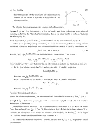
Remark Consider the function f : [0, 2] −→ R defined by
f (x) = −2x2 + 3x + 1.
The graph of f is shown in Figure 5.5. Although f (0) ≤ f (x) for all x sufficiently close to and greater 0, the
number 0 is not considered as a local minimizer of f .](https://image.slidesharecdn.com/basiccalculus-120628005326-phpapp02/85/Basic-calculus-140-320.jpg)
![134 Chapter 5. Applications of Differentiation
Example Let f : R −→ R be the function given by
f (x) = x3 − 3x2 + 3x.
d 3
Then we have f (x) = (x − 3x2 + 3x)
dx
= 3x2 − 6x + 3
= 3(x − 1)2 .
Thus f is differentiable on R. The number 1 is a critical number of f .
However, it is not a local extremizer of f since f is increasing on R. Figure 5.6
Suppose x0 is a critical number of a function f . At x0 , the function f may have a local maximum, a
local minimum or neither. The next result describes a simple way to determine which case it is using the first
derivative of f .
First Derivative Test Let f be a function that is differentiable on an open interval (a, b) and let x0 ∈ (a, b).
Suppose that x0 is a critical number of f .
(1) If f (x) changes from positive to negative as x increases through x0 , then x0 is a local maximizer of f .
(2) If f (x) changes from negative to positive as x increases through x0 , then x0 is a local minimizer of f .
(3) If f (x) does not change sign as x increases through x0 , then x0 is neither a local maximizer nor local
minimizer of f .
Explanation The assumption on x0 is that f (x0 ) = 0.
• The condition “ f (x) changes from positive to negative as x increases through x0 ” means that f (x) > 0
for x sufficiently close to and less than x0 and f (x) < 0 for x sufficiently close to and greater than x0 .
• The condition “ f (x) does not change sign as x increases through x0 ” means that f (x) is either always
positive or always positive for x sufficiently close and different from x0 .
Proof We give the proof for (1) and (3). The proof for (2) is similar to that for (1).
(1) If f (x) changes from positive to negative as x increases through x0 , then there is an open interval in the
form (a, x0 ) such that f (x) > 0 for all x ∈ (a, x0 ) and there is an open interval in the form (x0 , b) such
that f (x) < 0 for all x ∈ (x0 , b); hence by Theorem 5.1.1 and continuity, f is increasing on (a, x0 ] and
decreasing on [x0 , b). Therefore, f has a local maximum at x0 .
(3) If f (x) does not change sign as x increases through x0 , then there are open intervals in the form (a, x0 )
and (x0 , b) such that f (x) > 0 for all x ∈ (a, x0 ) ∪ (x0 , b) or f (x) < 0 for all x ∈ (a, x0 ) ∪ (x0 , b). In the
first case, by Theorem 5.1.1 f is increasing on (a, x0 ) as well as on (x0 , b) and hence by continuity, it is
increasing on (a, b). In the second case, f is decreasing on (a, b). Therefore, in any case, f does not have
a local extremum at x0 .
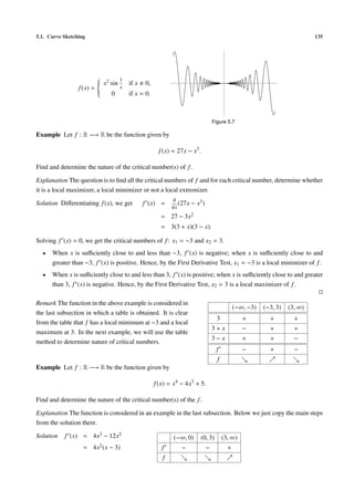
Remark For “nice” functions (for example, polynomials), the above result includes all possibilities. But we can
construct weird functions f such that x0 is a critical number of f and that f changes sign infinitely often on
the left and right of x0 . Figure 5.7 shows the graph of the function f given below; the number 0 is a critical
number of f .](https://image.slidesharecdn.com/basiccalculus-120628005326-phpapp02/85/Basic-calculus-142-320.jpg)
![136 Chapter 5. Applications of Differentiation
Solving f (x) = 0, we get the critical numbers of f : x1 = 0 and x2 = 3.
From the table, we see that
• the critical number x1 = 0 is not a local extremizer of f ;
• the critical number x2 = 3 is a local minimizer of f .
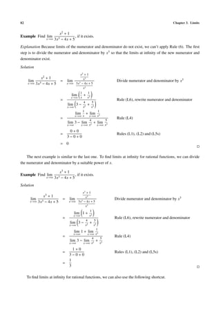
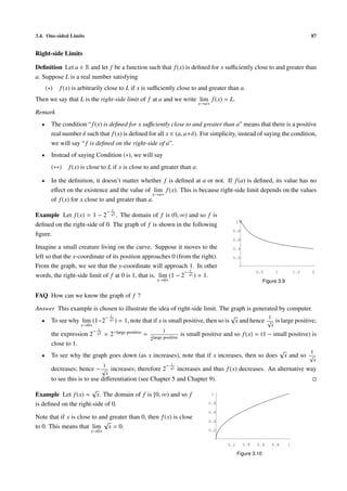
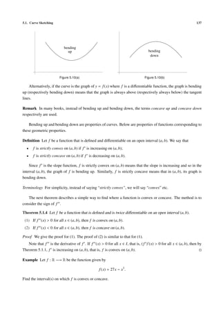
5.1.3 Convexity
In studying curves, we are also interested in finding out how the curves bend. Both curves shown in Figures
5.8(a) and (b) go up (as x goes from left to right). However the way how they bend are quite different.
Figure 5.8(a) Figure 5.8(b)
• In Figure 5.8(a), the curve goes up faster and faster, that is, the slope becomes more and more positive as
we move from left to right (the slope is increasing). We say that the curve is bending up.
• In Figure 5.8(b), although the curve goes up, the slope becomes less and less positive (the slope is
decreasing). We say that the curve is bending down.
Similarly we can consider curves that go down.
Figure 5.9(a) Figure 5.9(b)
• The curve in Figure 5.9(a) goes down. However, the slope becomes less and less negative. This means
that the slope is increasing and we say that the curve is bending up.
• The curve in Figure 5.9(b) also goes down. Moreover, the slope becomes more and more negative. This
means that the slope is decreasing and we say that the curve is bending down.
In summary, curves having shape shown in Figure 5.10(a) [or part of it] is said to be bending up and those
having shape shown in Figure 5.10(b) [or part of it] is said to be bending down.](https://image.slidesharecdn.com/basiccalculus-120628005326-phpapp02/85/Basic-calculus-144-320.jpg)
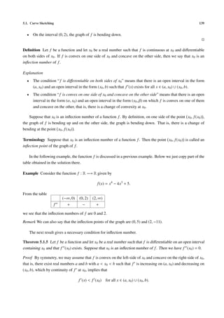
![138 Chapter 5. Applications of Differentiation
Explanation
• The question is to find maximal open interval(s), if any, on which f is convex or concave.
• The given function f is a “nice” function (a polynomial function). It can be differentiated any number
of times: f (n) (x) exists for all positive integers n and for all real numbers x. In particular, f is twice
differentiable on R. To apply Theorem 5.1.4, we have to solve inequalities f (x) > 0 and f (x) < 0.
This is done by setting up a table.
d
Solution Differentiating f (x), we get f (x) = (27x − x3 )
dx
= 27 − 3x2 .
d
Differentiating f (x), we get f (x) = (27 − 3x2 )
dx
(−∞, 0) (0, ∞)
= −6x.
−6 − −
x − +
• On the interval (−∞, 0), f is convex.
f + −
• On the interval (0, ∞), f is concave.
Remark
• When we consider “a function is convex/concave on an interval”, unlike increasing/decreasing, we do
not include the endpoint(s) of the interval. This is because the concept is defined for open intervals only.
Note that for a function f whose domain is a closed and bounded interval [a, b], f (x) is undefined when
x = a or b.
• There is a more general definition for convex/concave functions. The definition does not involve f and
it can be applied to closed intervals also.
Example Let f : R −→ R be the function given by
f (x) = x4 − 4x3 + 5.
Find where the graph of f is bending up or bending down.
Explanation This question is similar to the last one. The graph of f is bending up (or down) means that f is
convex (or concave). So we have to find intervals on which f is positive (or negative).
d 4
Solution Differentiating f (x), we get f (x) = (x − 4x3 + 5)
dx
= 4x3 − 12x2 .
d
Differentiating f (x), we get f (x) = (4x3 − 12x2 )
dx
(−∞, 0) (0, 2) (2, ∞)
= 12x2 − 24x
12x − + +
= 12x (x − 2).
x−2 − − +
f + − +
• On the intervals (−∞, 0) and (2, ∞), the graph of f is bending up.](https://image.slidesharecdn.com/basiccalculus-120628005326-phpapp02/85/Basic-calculus-146-320.jpg)
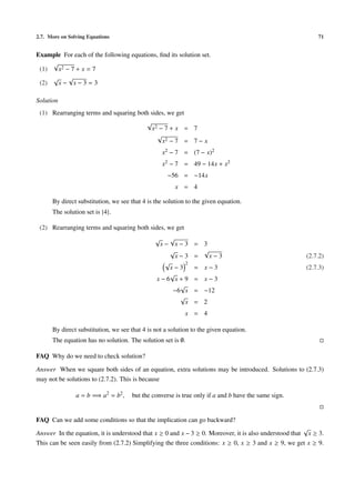
![5.1. Curve Sketching 143
5.1.4 Curve Sketching
Given a function f that is twice differentiable on an open interval (a, b), to sketch the graph of y = f (x) for
a < x < b, we can use the first derivative of f to find where the graph goes up or down and use the second
derivative of f to find where the graph bends up or down. Hence we can locate the local extremum points and
inflection points of the graph. Intercepts give additional information for the graph. If f is a rational function,
limits at infinity (±∞) and vertical asymptotes (infinite limits) are also useful.
The following table gives the shape of the graph of f corresponding to the four cases determined by the
signs of f and f . For example, first row first column corresponds to that both f and f are positive: the
figure indicates that the graph goes up and bends up.
f >0 f <0
f >0
f <0
Example Sketch the graph of y = 27x − x3 for x ∈ [−5.5, 5.5].
Explanation In the question, we are ask to draw the graph of f where f (x) = 27x − x3 for −5.5 ≤ x ≤ 5.5.
In the graph, we should locate the endpoints −5.5, f (−5.5) and 5.5, f (5.5) . In two previous examples, we
obtain the following:
(−∞, −3) (−3, 3) (3, ∞) (−∞, 0) (0, ∞)
f − + − f + −
The three numbers −3, 3 (zeros of f ) and 0 (zero of f ) divide R into four intervals: (−∞, −3), (−3, 0), (0, 3)
and (3, ∞). On each of these intervals, we can use the above tables to consider the signs of f and f .
Solution
(−∞, −3) (−3, 0) (0, 3) (3, ∞)
f − + + −
f + + − −
f
On the graph, we have
• Local minimum point −3, f (−3) = (−3, −54)
• Inflection point 0, f (0) = (0, 0)](https://image.slidesharecdn.com/basiccalculus-120628005326-phpapp02/85/Basic-calculus-151-320.jpg)
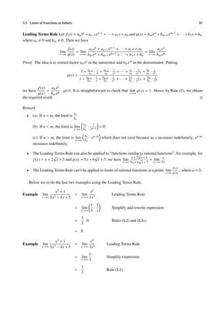
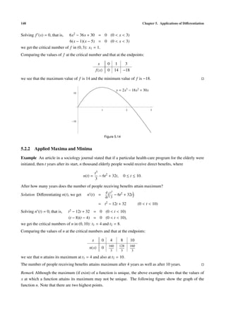
![5.2. Applied Extremum Problems 147
Recall (Extreme Value Theorem ) Let f : [a, b] −→ R be a continuous function. Then f attains its (absolute)
maximum and minimum. That is, there exist x1 , x2 ∈ [a, b] such that
f (x1 ) ≤ f (x) ≤ f (x2 ) for all x ∈ [a, b].
Note Extrema may occur at the endpoints a, b or at points in (a, b).
Figure 5.13 shows the graph of a function f with domain
[a, b]. Note that f attains its absolute minimum at x2 which
y = f (x)
belongs to the open interval (a, b) and attains its absolute max-
imum at b which is an endpoint. Also note that f has a relative
maximum at x1 but it does not attains its absolute maximum
there.
a x1 x2 b
Figure 5.13
Let f : [a, b] −→ R be a function that is differentiable on (a, b). Suppose that f attains its maximum or
minimum at x0 where a < x0 < b. Then by Theorem 5.1.3, x0 must be a critical number of f , that is, f (x0 ) = 0.
Thus we have the following procedures to find the absolute extrema of f .
Steps to find absolute extrema
(1) Find the critical number(s) of f in (a, b).
(2) Find the values of f at the endpoints a and b and that at the critical number(s) found in (1).
(3) The maximum and minimum values of f are, respectively, the greatest and smallest of the values found
in Step 2.
FAQ Do we need to check the nature (relative maximum or minimum) of the critical numbers?
Answer If you want to find absolute extrema, there is no need to check the nature of the critical numbers. Even
if you know that f has a local maximum (say) at a certain critical number x0 , you still have to compare values.
However if you know that f is increasing on [a, x0 ] and decreasing on [x0 , b], then you can tell that f attains
its absolute maximum at x0 , that is, f (x0 ) is the absolute maximum; and to get the absolute minimum, you can
compare the values f (a) and f (b).
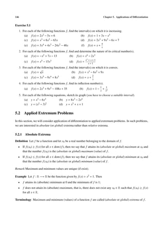
Example Find the absolute extremum values of the function f given by
f (x) = 2x3 − 18x2 + 30x
on the closed interval [0, 3].
Explanation In this question, the domain of f is taken to be [0, 3]. Since f is continuous on [0, 3], it follows
from the Extreme Value Theorem that f attains its absolute extrema. Note that f is differentiable on (0, 3).
Thus we can apply the above steps to find the absolute extremum values.
d
Solution Differentiating f (x), we get f (x) = (2x3 − 18x2 + 30x)
dx
= 6x2 − 36x + 30 (0 < x < 3)](https://image.slidesharecdn.com/basiccalculus-120628005326-phpapp02/85/Basic-calculus-155-320.jpg)
![150 Chapter 5. Applications of Differentiation
Differentiating A(x), we get A (x) = 10 − 2x (0 < x < 10).
Solving A (x) = 0, we obtain the critical number of A: x1 = 5. Comparing the values of A at the critical number
and that at the endpoints:
x 0 5 10
A(x) 0 25 0
we see that A attains its maximum at x1 = 5. Hence the dimensions of the largest rectangle is 5 cm × 5 cm.
FAQ Can we apply the Second Derivative Test to check that A has maximum at x1 = 5?
Answer If you use the Second Derivative Test, you can only tell that A has local maximum at x1 = 5. In this
problem, we want global maximum.
However, there is a special version of the Second Derivative Test which can be applied to this problem.
Second Derivative Test (Special Version) Let f be a function and let x0 be a real number such that f is
differentiable on an open interval (a, b) containing x0 . Suppose that x0 is the only critical number of f in (a, b).
(1) If f (x0 ) < 0, then in (a, b), f attains its maximum at x0 , that is, f (x0 ) ≥ f (x) for all x ∈ (a, b).
(2) If f (x0 ) > 0, then in (a, b), f attains its minimum at x0 , that is, f (x0 ) ≤ f (x) for all x ∈ (a, b).
Explanation Below we give a proof for (1). For this, we use a method called Proof by Contradiction. The result
we want to prove is in the form “Assumption; Conclusion”.
• The assumption is “ f is differentiable on an open interval (a, b) containing x0 and x0 is the only critical
number of f in (a, b)”.
• The conclusion is “If f (x0 ) < 0, then in (a, b), f attains its maximum at x0 ”.
The negation (opposite) of the conclusion is “It is not true that if f (x0 ) < 0, then in (a, b), f attains its
maximum at x0 ” which can be restated as “ f (x0 ) < 0 and in (a, b), f does not attain its maximum at x0 ”.
The method of Proof by Contradiction is to assume that the conclusion is false and use it (together with the
given assumption) to deduce something that contradicts the given assumption. More specifically, we want to
deduce that there exists x2 ∈ (a, b) with x2 x0 such that f (x2 ) = 0, which contradicts the assumption that x0
is the only critical number of f in (a, b).
In the proof below, we write “Without loss of generality, we may assume that x1 > x0 ”. It means that the
other case where x1 < x0 can be treated similarly.
Proof We give a proof for (1). For (2), it can be proved similarly or alternatively proved by applying (1) to the
function − f .
Suppose that (1) does not hold, that is, suppose that f (x0 ) < 0 but there exists x1 ∈ (a, b) such that
f (x1 ) > f (x0 ).
Without loss of generality, we may assume that x1 > x0 . Applying the Extreme Value Theorem to f on the
interval [x0 , x1 ], we see that there exists x2 ∈ [x0 , x1 ] such that
f (x2 ) ≤ f (x) for all x ∈ [x0 , x1 ].](https://image.slidesharecdn.com/basiccalculus-120628005326-phpapp02/85/Basic-calculus-158-320.jpg)
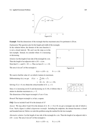
![5.2. Applied Extremum Problems 153
Since V (3) = −72 < 0 and x1 = 3 is the only critical number of V in (0, 9), it follows from the Second
Derivative Test (Special Version) that in (0, 9), V attains its maximum at x1 = 3. Thus the length of the side of
the square that must be cut off is 3 cm and the maximum volume is V(3) = 432 cm3 .
400
V = x(18 − 2x)2
300
200
100
2 4 6 8
Figure 5.19
5.2.3 Applications to Economics
Suppose a manufacturer produces and sells a product. Denote C(q) to be the total cost for producing and
marketing q units of the product. Thus C is a function of q and it is called the (total) cost function. The rate of
change of C with respect to q is called the marginal cost, that is,
dC
marginal cost = .
dq
Denote R(q) to be the total amount received for selling q units of the product. Thus R is a function of q and it
is called the revenue function. The rate of change of R with respect to q is called the marginal revenue, that is,
dR
marginal revenue = .
dq
Denote P(q) to be the profit of producing and selling q units of the product, that is,
P(q) = R(q) − C(q).
Thus P is a function of q and it is called the profit function.
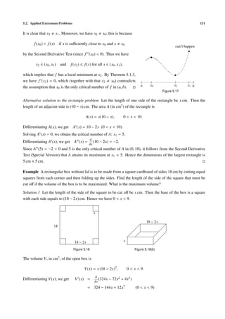
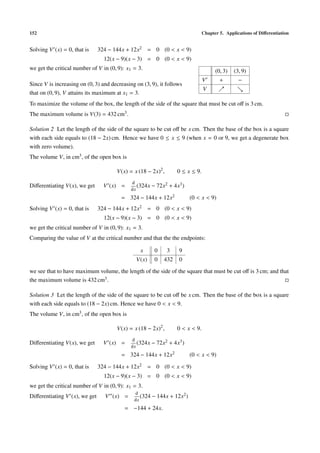
Denote qmax to be the largest number of units of the product that the manufacturer can produce. Assuming
that q can take any value between 0 and qmax . Then for each of the functions C, R and P, the domain is
[0, qmax ]. Suppose that the cost function and the revenue function are differentiable on (0, qmax ) and suppose
that producing 0 or qmax units of the product will not give maximum profit. Then in order to have maximum
profit, we need
dP
= 0,
dq
or equivalently,
dC dR
= ,
dq dq
that is, marginal cost = marginal revenue.
Example The demand equation for a certain product is
q − 90 + 2p = 0, 0 ≤ q ≤ 90,](https://image.slidesharecdn.com/basiccalculus-120628005326-phpapp02/85/Basic-calculus-161-320.jpg)
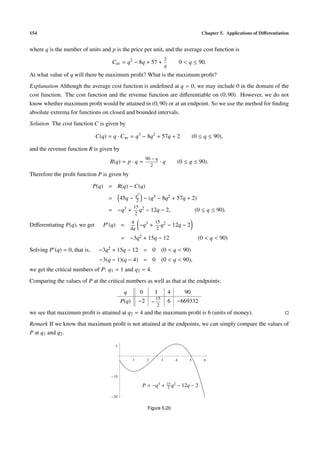
![5.2. Applied Extremum Problems 155
Exercise 5.2
1. For each of the given function f , find its absolute extrema on the given interval.
(a) f (x) = 4x3 + 3x2 − 18x + 1, [0, 3]
(b) f (x) = −3x5 + 5x3 + 2, [−2, 0]
(c) f (x) = 1 + 2x 3 − 3x4 , [−1, 1]
2. Find two positive real numbers whose sum is 50 and whose product is a maximum.
3. Find two real numbers x and y satisfying 2x + y = 15 such that x2 + y2 is minimized.
Can you find a geometric meaning for the result?
4. Find the dimensions of the rectangle of area 100 square units that has the least perimeter.
5. A rectangular field is to be enclosed by a fence and divided equally into two parts by a fence parallel to
one pair of the sides. If a total of 600 m of fence is to be used, find the dimensions of the field if its area
is to be maximized.
6. A book is to contain 36 in2 of printed matter per page, with margins of 1 in along the sides and 1 1 in
2
along the top and bottom. Find the dimensions of the page that will require the minimum amount of
paper.
7. Suppose that a ball is thrown straight up into the air and its height after t seconds is 5 + 24t − 16t2 feet.
Determine how long it will take the ball to reach its maximum height and determine the maximum height.
8. It is known from experiments that the height (in meter) of a certain plant after t months is given (approx-
imately) by
√
h(t) = t − t, 0 ≤ t ≤ 1.
How long, on the average, will it take a plant to reach its maximum height? What is the maximum height?
9. A company manufactures and sells x pieces of a certain product per month. The monthly cost (in dollars)
is
C(x) = 120000 + 100x
and the price-demand equation is
x
p = 300 −
15
where 0 ≤ x ≤ 4000. Find the maximum profit, the production level that will give the maximum profit,
and the price the company should charge for each piece of the product.](https://image.slidesharecdn.com/basiccalculus-120628005326-phpapp02/85/Basic-calculus-163-320.jpg)
![Chapter 6
Integration
6.1 Definite Integrals
In the introduction of Chapter 3, we consider the area of the region under the curve y = x2 and above the x-axis
for x between 0 and 1. To get approximations for the area, we divide [0, 1] into n equal subintervals:
[x0 , x1 ], [x1 , x2 ], ..., [xn−1 , xn ],
i
where xi = for 0 ≤ i ≤ n; and for each i = 1, . . . , n, in the subinterval [xi−1 , xi ], we take the left endpoint xi−1
n
n 1 1 1
and consider the sum f (xi−1 ) · , that is, f (x0 ) · + · · · + f (xn−1 ) · . We have seen that the sum is close to
i=1 n n n
1
(which is the required area) if n is large. Using limit notation, the result can be written as
3
n
1 1
lim f (xi−1 ) · = . (6.1.1)
n→∞
i=1
n 3
The above idea can be generalized to any continuous functions f on any closed and bounded interval. Moreover,
f need not be non-negative.
Theorem 6.1.1 Let f be a function that is continuous on a closed and bounded interval [a, b]. Then the follow-
ing limit exists:
n
b−a
lim f (xi−1 ) · ,
n→∞
i=1
n
i
where xi = a + (b − a) for 0 ≤ i ≤ n.
n
Explanation
y = f (x)
• By the construction of the xi ’s, we have x0 = a, xn = b,
x0 < x1 < · · · < xn , and for every i = 1, . . . , n, the
b−a
subinterval [xi−1 , xi ] has length and xi−1 is the left-
n
endpoint of the subinterval.
• If f is non-negative on [a, b], that is, f (x) ≥ 0 for all
n b−a
x ∈ [a, b], then lim f (xi−1 )· is the area bounded
n→∞ i=1 n
x0 x1 ··· xn−1 xn
by the graph of f , the x-axis and the vertical lines given
by x = a and x = b. Figure 6.1](https://image.slidesharecdn.com/basiccalculus-120628005326-phpapp02/85/Basic-calculus-165-320.jpg)
![158 Chapter 6. Integration
Definition Let f be a function that is continuous on a closed and bounded interval [a, b]. The number
n b−a i
lim f (xi−1 ) · , where xi = a + (b − a) for 0 ≤ i ≤ n, is called the definite integral of f from a to
n→∞ i=1 n n
b
b and is denoted by a
f (x) dx, that is,
b n
b−a
f (x) dx = lim f (xi−1 ) · . (6.1.2)
a n→∞
i=1
n
Example The result given in (6.1.1) can be written as
1
1
x2 dx = . (6.1.3)
0 3
Remark In Theorem 6.1.1, in each subinterval [xi−1 , xi ], instead of taking the left endpoint xi−1 , we can take
the right endpoint xi (see Figure 6.2) and we have
n b
b−a
lim f (xi ) · = f (x) dx. (6.1.4)
n→∞
i=1
n a
y = f (x) y = f (x)
x0 x1 ··· xn−1 xn x0 t1 x1 t2 ··· tn xn
Figure 6.2 Figure 6.3
n b−a
In fact, we can take an arbitrarily point (denoted by ti ) in [xi−1 , xi ]: the sum f (ti ) · is close to
i=1 n
b
a
f (x) dx if n is large enough (see Figure 6.3).
More generally, the subintervals [x0 , x1 ], . . . , [xn−1 , xn ] need not be of equal lengths. All we need is that the
lengths are small enough: if a = x0 < x1 < · · · < xn = b and ∆x1 , . . . , ∆xn are small enough, where ∆xi is the
length of the ith subinterval [xi−1 , xi ], then for every choice of t1 , . . . , tn with ti ∈ [xi−1 , xi ] for 1 ≤ i ≤ n, the
sum (called a Riemann Sum)
n
f (ti )∆xi
i=1
b
is close to a
f (x) dx. Many authors use this to define definite integral.
Below, we apply (6.1.4) to deduce the result given in (6.1.3). For this, we take f (x) = x2 , a = 0, b = 1 and
i
xi = for 0 ≤ i ≤ n.
n](https://image.slidesharecdn.com/basiccalculus-120628005326-phpapp02/85/Basic-calculus-166-320.jpg)
![6.1. Definite Integrals 159
Example By (6.1.4), we have
1 n 2
i 1
x2 dx = lim ·
0 n→∞
i=1
n n
n
1
= lim i2
n→∞ n3
i=1
1 n(n + 1)(2n + 1)
= lim 3 · Sum of Squares Formula
n→∞ n 6
2n3
= lim Leading Term Rule
n→∞ 6n3
1
=
3
b
FAQ Can we define a
f (x) dx if f is not continuous on [a, b]?
b
Answer In defining a
f (x) dx, we need Theorem 6.1.1. The condition “ f is continuous on [a, b]” is used to
n 1
guarantee that lim f (xi−1 ) · exists.
n→∞ i=1 n
In general, if f is a function defined on [a, b] such that there exists a (unique) real number I satisfying
n
(∗) f (ti )∆xi is arbitrarily close I if ∆x1 , . . . , ∆xn are sufficiently small, where ∆xi = xi − xi−1 for 1 ≤ i ≤ n,
i=1
a = x0 < x1 < · · · < xn = b and ti ∈ [xi−1 , xi ] for 1 ≤ i ≤ n,
b
then the unique number I is defined to be a
f (x) dx.
Remark
• In view of (∗), we may write
b n
f (x) dx = lim f (ti )∆xi ,
a ∆ →0
i=1
where ∆ → 0 means the lengths ∆xi ’s tend to zero. However, this kind of limit is different from that
discussed in Chapter 3.
• The symbol was introduced by Leibniz and is called the integral sign. It is an elongated S and was
chosen because a definite integral is a limit of sums.
• Since the definite integral of a (continuous) function on [a, b] depends on the function f and the interval
b
[a, b] only, it can simply be denoted by a f , omitting the variable x and the notation dx. However, the
b
notation a
f (x) dx is preferred. There are two reasons:
n
(1) the notation dx reminds us of the factors ∆xi in the sums f (ti )∆xi ;
i=1
(2) with the variable included in the notation, it is easier to handle the substitution method for integra-
tion (see Chapter 10).
b
• In the notation a
f (x) dx, the variable x is called a dummy variable; it can be replaced by any other
1 2 1
symbol. For example, using t as the dummy variable, (6.1.3) can be written as 0
t dt = . Note that if
3
we use t as the dummy variable, we have to change dx to dt accordingly.](https://image.slidesharecdn.com/basiccalculus-120628005326-phpapp02/85/Basic-calculus-167-320.jpg)
![160 Chapter 6. Integration
2
Example Use definition to find x dx.
1
i
Solution Applying (6.1.2) to f (x) = x, a = 1, b = 2 and xi = 1 + for 0 ≤ i ≤ n, we get
n
2 n
i−1 1
x dx = lim 1+ ·
1 n→∞
i=1
n n
n
1
= lim 2 (n + i − 1)
n→∞ n
i=1
1 n(n + 2n − 1)
= lim 2 · Sum of A.P.
n→∞ n 2
3n − 1
= lim
n→∞ 2n
3n
= lim Leading Term Rule
n→∞ 2n
3
= .
2
Remark The value of the definite integral is the area of the trapezoidal region 2
shown in Figure 6.4. Readers can check that the result agrees with that obtained
1
by using formula for area of trapezoid.
1 2
Figure 6.4
Definite Integral for Constant Functions Let c be a constant and let a and b be real numbers with a < b. Then
b
we have c dx = c · (b − a).
a
i
Proof Applying (6.1.2) to f (x) = c and xi = a + (b − a) for 0 ≤ i ≤ n, we get
n
b n
b−a
c dx = lim c·
a n→∞
i=1
n
b−a
= lim c · ×n Sum of Constants
n→∞ n
= lim c · (b − a) Rule (L1) for Limit
n→∞
= c · (b − a)
b c
Remark If c > 0, then a
c dx is the area of the rectangular region shown in
Figure 6.5.
a b
Figure 6.5
Rules for Definite Integrals Let f and g be functions that are continuous on a closed and bounded interval
[a, b]. Let α be a constant and let c ∈ (a, b). Then we have](https://image.slidesharecdn.com/basiccalculus-120628005326-phpapp02/85/Basic-calculus-168-320.jpg)
![6.1. Definite Integrals 161
b b b
(Int1) f (x) + g(x) dx = f (x) dx + g(x) dx
a a a
Proof Apply definition and Rule (L4) for limits of sequences.
b b
(Int2) α f (x) dx = α f (x) dx
a a
Proof Apply definition and Rule (L5s) for limits of sequences.
Remark Using Rules (Int1) and (Int2), we get
b b b
f (x) − g(x) dx = f (x) dx − g(x) dx.
a a a
In fact, Rule (Int1) is valid for sum and difference of finitely many (continuous) functions.
b c b
y = f (x)
(Int3) f (x) dx = f (x) dx + f (x) dx.
a a c
Explanation The proof for the result is not easy. For the case where
f is nonnegative on [a, b], the result can be seen from the geometric
interpretation shown in Figure 6.6.
a c b
Figure 6.6
1 1
Example 5x2 dx = 5 x2 dx Rule (Int2)
0 0
1
= 5× by (6.1.3)
3
5
=
3
2 2 2
Example (3 − x) dx = 3 dx − x dx Rule (Int1)
1 1 1
3 Definite Integral for Constant &
= 3 × (2 − 1) −
2 Example on Page 160
3
=
2
b
In defining a
f (x) dx, we need a < b. For convenience, we introduce the following:
Convention Let f be a function that is continuous on a closed and bounded interval [a, b] and let c ∈ [a, b].
Then we define
a b
(1) f (x) dx = − f (x) dx
b a
c
(2) f (x) dx = 0
c](https://image.slidesharecdn.com/basiccalculus-120628005326-phpapp02/85/Basic-calculus-169-320.jpg)
![162 Chapter 6. Integration
2
Example (1 + 2x − 3x2 ) dx = 0 since the function 1 + 2x − 3x2 is continuous on [0, 3] (for example)
2
and 2 ∈ [0, 3].
0 1
Example x2 dx = − x2 dx by convention
1 0
1
= − by (6.1.3)
3
b
Terminology In a definite integral a
f (x) dx,
• the function f is called the integrand;
• the numbers a and b are called the limits of integration; a is the lower limit and b the upper limit.
Exercise 6.1
1. For each of the following definite integrals, use the results in this section to find its value:
1 1
(a) 0
(1 − 3x2 ) dx (b) 2
4x dx
1
2. Use definition to find the definite integral 0 x3 dx.
n2 (n + 1)2
Given: 13 + 23 + · · · + n3 =
4
6.2 Fundamental Theorem of Calculus
In the last section, we give the definition and some examples of definite integral. Although we have some
rules that are useful in calculating definite integrals, we still have to know the definite integrals of some “basic
functions”. For example, using rules, we can find the definite integrals of polynomials provided that we know
b n
a
x dx for positive integers n. Finding definite integrals by first principle (that is, by definition) is very
tedious. In this section, we describe a simple way (Fundamental Theorem of Calculus, Version 2) to find
definite integrals. It is quite surprising that differentiation and integration are related— they are reverse process
of each other (see Fundamental Theorem of Calculus, Versions 1 and 3).
Given a function f that is continuous on a closed and bounded interval [a, b], in order to “find” the definite
b
integral a f (x) dx, we introduce an auxiliary function F from [a, b] into R defined by
x
F(x) = f (t) dt a ≤ x ≤ b.
a
In the construction of F, for each x ∈ (a, b], the value F(x) is defined
to be the definite integral of f over the interval [a, x] and for x = a, by
a
convention, F(a) = a f (t) dt is defined to be 0. Note that x is used as the
independent variable for the function F. For clarity, we use another symbol
t as the dummy variable for the definite integral of f over [a, x].
Geometrically, if f is nonnegative on [a, b], then F can be considered as an
a x b
“area function” with F(x) equal to the area under the graph of f (and above
Figure 6.7
the horizontal axis) from a to x.](https://image.slidesharecdn.com/basiccalculus-120628005326-phpapp02/85/Basic-calculus-170-320.jpg)
![6.2. Fundamental Theorem of Calculus 163
By the construction of F, the required definite integral is F(b). If we can find a formula for F(x), then we
can solve the problem. The following result gives a relation between F and f .
Fundamental Theorem of Calculus, Version 1 Let f be a function that is continuous on a closed and bounded
interval [a, b]. Let F be the function from [a, b] into R defined by
x
F(x) = f (t) dt for a ≤ t ≤ b.
a
Then F is continuous on [a, b] and differentiable on (a, b) with F (x) = f (x) for all x ∈ (a, b).
Explanation The proof of this result will be given in the appendix. Below we explain how to “obtain” F = f
on (a, b) intuitively for the case where f is nonnegative on [a, b]. Recall that
F(x + h) − F(x)
F (x) = lim .
h→0 h
For x ∈ (a, b) and for sufficiently small h > 0 (such that a + h ≤ b), we have
x+h x
F(x + h) − F(x) = f (t) dt − f (t) dt by construction of F
a a
x x+h x
= f (t) dt + f (t) dt − f (t) dt Rule (Int3)
a x a
x+h
= f (t) dt.
x
x+h
Note that x f (t) dt is the area of the region below the graph
of f (and above the horizontal axis) from x to x + h. If h is
small, then [x, x+h] is a short interval and the area of the small
region under consideration can be approximated by the area of
the rectangular region with base [x, x+h] on the horizontal axis
and height equal to f (x). Thus we have a x x+h b
Figure 6.8
x+h
f (t) dt is close to f (x) · h if h is small,
x
from which we obtain
x+h
F(x + h) − F(x) x
f (t) dt
= is close to f (x) if h is small.
h h
Taking limit, we get F (x) = f (x).
F(x + h) − F(x)
Remark To be more precise, the above argument gives lim = f (x) only.
h→0+ h
b
In view of the Fundamental Theorem of Calculus (Version 1), to find a
f (x) dx, we should look for func-
tions G such that G = f .
Definition Let f be a function that is continuous on a closed and bounded interval [a, b]. Suppose that G is a
function that is defined on [a, b] such that the following two conditions are satisfied:](https://image.slidesharecdn.com/basiccalculus-120628005326-phpapp02/85/Basic-calculus-171-320.jpg)
![164 Chapter 6. Integration
(1) G is continuous on [a, b];
(2) G is differentiable on (a, b) and G (x) = f (x) for all x ∈ (a, b).
Then we say that G is a primitive for f on [a, b].
Example Let f (x) = 3x2 and let G(x) = x3 . Note that f and G are continuous on R and that G (x) = f (x) for
all x ∈ R. Thus G is a primitive for f on every closed and bounded interval [a, b].
Remark Primitive is not unique. For example, the function G1 (x) = x3 + 1 is also a primitive for f (on every
closed and bounded interval). In fact, for every constant C, the function
x3 + C (6.2.1)
is a primitive for f (on every closed and bounded interval). It is natural to ask whether there are any more
primitives:
• If F (x) = f (x) for all x ∈ R, must F be in the form (6.2.1)?
Corollary 6.2.2, which is based on the following theorem, tells that the answer is affirmative.
Theorem 6.2.1 Let F and G be functions that are defined on a closed and bounded interval [a, b]. Suppose that
F and G are continuous on [a, b] and are differentiable on (a, b) with F (x) = G (x) for all x ∈ (a, b). Then on
[a, b], the functions F and G differ by a constant, that is, there exists a constant C such that
F(x) − G(x) = C for all x ∈ [a, b].
Explanation The following is the geometry meaning of the result:
• The condition “F (x) = G (x) for all x ∈ (a, b)” means that at corresponding points (same x-coordinates),
tangents to the graphs of F and G are parallel.
• The conclusion is that the graph of F can be obtained from that of G by moving it upward (C > 0) or
downward (C < 0).
Proof Let f be the function from [a, b] into R defined by
f (x) = F(x) − G(x).
Note that f (x) = F (x) − G (x) = 0 for all x ∈ (a, b). Hence by Theorem 5.1.1, there exists a constant C such
that
f (x) = C for all x ∈ (a, b).
Since f is continuous on [a, b], it follows that
f (x) = C for all x ∈ [a, b]
from which we get the required result.
Corollary 6.2.2 Let f be a function that is continuous on a closed and bounded interval [a, b]. Suppose that F
and G are primitives for f on [a, b]. Then on [a, b], the functions F and G differ by a constant.](https://image.slidesharecdn.com/basiccalculus-120628005326-phpapp02/85/Basic-calculus-172-320.jpg)
![6.2. Fundamental Theorem of Calculus 165
Proof This is an immediate consequence of Theorem 6.2.1 since by the definition of primitive, the functions
F and G are continuous on [a, b] and differentiable on (a, b) and F (x) = f (x) = G (x) for all x ∈ (a, b).
2
Example Find the value of the definite integral 3x2 dx.
1
Solution Let f (x) = 3x2 and let G(x) = x3 . Then G is a primitive for f on [1, 2].
By the Fundamental Theorem of Calculus (Version 1), the function F given by
x
F(x) = 3t2 , dt, 1 ≤ x ≤ 2.
1
is a primitive for f on [1, 2].
By Corollary 6.2.2, on the interval [1, 2], the functions F and G differ by a constant, that is, there exists a
constant C such that
F(x) − x3 = C for all x ∈ [1, 2].
Putting x = 1 and using the construction of F, we get
0 − 1 = C.
which implies that F(x) = x3 − 1 for all x ∈ [1, 2]. Hence, we have
2
3x2 dx = F(2) by construction of F
1
= 23 − 1
= 7.
Remark The above procedure can be used to find the definite integral of f on any closed and bounded interval
[a, b]. This is because G is a primitive for f on every [a, b].
From the above example, we see that given a function f that is continuous on a closed and bounded interval
b
[a, b], if we can find a primitive for f over [a, b], then we can find the definite integral a f (x) dx. The following
b
result describe an alternative procedure for finding a
f (x) dx (there is no need to find the constant C).
Fundamental Theorem of Calculus, Version 2 Let f be a function that is continuous on a closed and bounded
interval [a, b]. Suppose that G is a primitive for f on [a, b]. Then we have
b
f (x) dx = G(b) − G(a).
a
Proof Let F be the function from [a, b] into R defined by
x
F(x) = f (t) dt, a ≤ x ≤ b.
a
By the Fundamental Theorem of Calculus, Version 1, the function F is a primitive for f on [a, b]. Hence by
Corollary 6.2.2, there exists a constant C such that
F(x) − G(x) = C for all x ∈ [a, b]. (6.2.2)](https://image.slidesharecdn.com/basiccalculus-120628005326-phpapp02/85/Basic-calculus-173-320.jpg)
![166 Chapter 6. Integration
Therefore, we have
b
f (x) dx = F(b) by construction of F
a
= F(b) − F(a) since F(a) = 0
= G(b) + C − G(a) + C by (6.2.2)
= G(b) − G(a)
Below we redo the last example using the second version of the Fundamental Theorem of Calculus.
2
Example Evaluate 3x2 dx
1
Solution Since the function G(x) = x3 is a primitive for the function 3x2 on the interval [1, 2], it follows from
the Fundamental Theorem of Calculus (Version 2) that
2
3x2 dx = G(2) − G(1)
1
= 23 − 13
= 7.
FAQ Can we use other primitives for f ?
Answer The Fundamental Theorem tells that any primitive will work. Try it yourselves.
Notation We will use the notation G(b) − G(a) quite often. For simplicity, it will be denoted by
b b
G(x) or G(x) .
a a
5
Example Find 2x dx.
3
b
Explanation To find a f (x) dx, in applying the Fundamental Theorem of Calculus (Version 2), we have to find
a function G that is continuous on [a, b] such that G = f on (a, b). In this course, functions that we considered
are “nice”—there is no need to check continuity; we just need to check that G = f (usually valid on a much
larger interval).
Solution By inspection, we see that the function x2 is a primitive for the integrand 2x (on every closed and
bounded interval). Thus by the Fundamental Theorem of Calculus (Version 2), we have
5 5
2x dx = x2
3 3
= 52 − 32
= 16.
Remark The definite integral is the area of the trapezoidal region that lies below the line y = 2x, above the
x-axis and is bounded on the left and right by the vertical lines x = 3 and x = 5. Use formula to check the
answer yourselves.](https://image.slidesharecdn.com/basiccalculus-120628005326-phpapp02/85/Basic-calculus-174-320.jpg)
![6.3. Indefinite Integrals 167
Exercise 6.2
1. For each of the following functions f , use inspection to find a primitive. Is your answer a primitive for f
on every closed and bounded interval [a, b]? If not, what can you tell about [a, b]?
(a) f (x) = x (b) f (x) = 1
(c) f (x) = x5 (d) f (x) = 2x + 1
1 √
(e) f (x) = √ (f) f (x) = x
2 x
2. Use inspection to find a primitive for f (x) = x4 and hence evaluate the following definite integrals.
1 4 3 4
(a) 0
x dx (b) 1
x dx
3 4 3
(c) 0
x dx (d) 0
7x4 dx
6.3 Indefinite Integrals
Suppose that f and F are functions that are continuous on a closed and bounded interval [a, b]. To show that F
is a primitive for f on [a, b] means to show that F (x) = f (x) for all x ∈ (a, b). In view of this, we introduce a
concept similar to primitive.
Definition Let f be a function that is continuous on an open interval (a, b). Suppose F is a function defined on
(a, b) such that F (x) = f (x) for all x ∈ (a, b). Then we say that F is an antiderivative for f on (a, b).
Example
1
(1) Let f (x) = x2 and let F(x) = x3 . Then we have
3
F (x) = f (x) for all x ∈ R.
Thus F is an antiderivative for f on every open interval contained in R.
1 √
(2) Let g(x) = √ and let G(x) = 2 x. Then we have
x
G (x) = g(x) for all x > 0.
Thus G is an antiderivative for g on every open interval contained in (0, ∞).
Remark Suppose that F is an antiderivative for f on (a, b). Then F is a primitive for f on every closed and
bounded interval [c, d] contained in (a, b). If in addition, F and f are defined at a and b and are continuous on
[a, b], then F is a primitive for f on [a, b].
The following result is similar to that given in Corollary 6.2.2.
Theorem 6.3.1 Let f be a function that is continuous on an open interval (a, b). Suppose that F and G are
antiderivatives for f on (a, b). Then on (a, b), the functions F and G differ by a constant.
Proof Apply the proof (the first part) for Theorem 6.2.1](https://image.slidesharecdn.com/basiccalculus-120628005326-phpapp02/85/Basic-calculus-175-320.jpg)
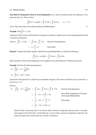
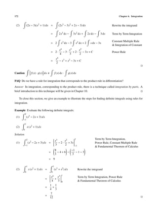
![6.4. Application of Integration 173
Exercise 6.3
1. Perform the following integration:
4
(a) 2x5 dx (b) 3 − √ dx
x
√
(c) (x7 − 3x + 2) dx (d) (x2 − x + 3) dx
2
(e) √ dx (f) (x2 − 5x + 1)(2 − 3x) dx
3x x
x2 + 1
(g) (x2 − 3)2 dx (h) dx
x2
2. Evaluate the following definite integrals:
3 3
(a) 0
2x3 dx (b) −3
2x3 dx
2 2 4
(c) −1
(1 − 5x4 ) dx (d) 0
(x − 3x2 + 5) dx
2 4 4 2 1
(e) −2
(x − 3x2 + 5) dx (f) 1
x + √ dx
2 x
2 x2 + 1 2
(g) 1
√ dx (h) 0
x (2 − 3x)2 dx
x
6.4 Application of Integration
y = f (x)
Area under Graph of Function Let f be a function that is continuous
on a closed and bounded interval [a, b]. Suppose that f is nonnegative
on [a, b]. Then the area A of the region that lies below the graph of f
A
and above the x-axis from x = a to x = b is given by
b
A= f (x) dx. a b
a Figure 6.9
Example Find the area of the region that is bounded by the curve
√ R2
y = x, the line x = 1 and the x-axis.
R1
Explanation The curve, the vertical line and the x-axis divide the R3 R4
plane into six regions—five of them are unbounded (R1 , R2 , R4 , R5 R5 R6
and R6 ) and one of them is bounded (R3 , the required one). Figure 6.10a
√
Solution Let f (x) = x. The region under consideration lies below the graph of f and above the x-axis from
x = 0 to x = 1. The required area A is
1
A = f (x) dx √
0 y= x
1
1
= x 2 dx
0
3 1 A
x2
= 3
2 0 1
2 Figure 6.10b
= (square units).
3](https://image.slidesharecdn.com/basiccalculus-120628005326-phpapp02/85/Basic-calculus-181-320.jpg)
![174 Chapter 6. Integration
Area between Graphs of Functions Let f and g be functions
that are continuous on a closed and bounded interval [a, b]. Sup-
pose that f (x) ≤ g(x) for all x ∈ [a, b] (this means that the graph
y = g(x)
of f lies below that of g). Then the area A of the region that is
bounded by the graphs of f and g and the vertical lines x = a and
A
x = b is given by
b y = f (x)
A= g(x) − f (x) dx.
a
a b
Figure 6.11
Proof For the case where f is nonnegative (hence the graphs of both f and g are above the x-axis), we have
A = Ag − A f , where Ag (respectively A f ) is the area of the region that lies below the graph of g (respectively
the graph of f ) and above the x-axis from x = a to x = b (see Figure 6.12a). Hence, using rules for definite
integrals (Int1) and (Int2), we have
b b b
A= g(x) dx − f (x) dx = g(x) − f (x) dx.
a a a
y = g1 (x)
y = f1 (x)
Ag y = g(x)
Af
a b y = f (x)
Figure 6.12a
Figure 6.12b
For the general case, we can move the region upward suitably so that the graph of f is above the x-axis and
then apply the result for the case where f is nonnegative (see Figure 6.12b). Indeed, since f is continuous on
[a, b], there exists a constant k such that f (x) + k ≥ 0 for all x ∈ [a, b]. Let f1 and g1 be the functions from [a, b]
into R given by
f1 (x) = f (x) + k and g1 (x) = g(x) + k for a ≤ x ≤ b.
Since area is translation invariant, the required area A is equal to the area of the region that is bounded by the
graphs of f1 and g1 and the vertical lines x = a and x = b. Hence by what we obtain for the special case (since
f1 is nonnegative), we have
b b
A= g1 (x) − f1 (x) dx = g(x) − f (x) dx.
a a
Example Find the area of the region bounded by the parabola y = x2 and the line y = x + 2.](https://image.slidesharecdn.com/basiccalculus-120628005326-phpapp02/85/Basic-calculus-182-320.jpg)
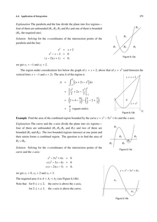
![176 Chapter 6. Integration
Therefore, we have
2 3
A = (x3 − 5x2 + 6x) − 0 dx + 0 − (x3 − 5x2 + 6x)] dx
0 2
2 3
x4 5x3 x4 5x3
= − + 3x2 − − + 3x2
4 3 0 4 3 2
8 9 8
= −0 − −
3 4 3
37
= .
12
Next we will give some examples that can be done using definite integrals as well as indefinite integrals.
Before that, we give a result that is also known as the Fundamental Theorem of Calculus.
Fundamental Theorem of Calculus, Version 3 Let f be a function such that f is continuous on an open
interval (a, b). Then for every x0 ∈ (a, b), we have
x
f (x) = f (t) dt + f (x0 ) for all x ∈ (a, b).
x0
Proof Let g be the function from (a, b) into R defined by
x
g(x) = f (t) dt for a < x < b.
x0
From the Fundamental Theorem of Calculus (Version 1), we see that g is an antiderivative for f on (a, b). Since
f is also an antiderivative of f on (a, b), it follows from Theorem 6.3.1 that there exists a constant k such that
f (x) − g(x) = k for all x ∈ (a, b).
x0
Putting x = x0 , we get f (x0 ) − g(x0 ) = k which yields k = f (x0 ) since g(x0 ) = x0
f (t) dt = 0. Therefore we
have
f (x) = g(x) + f (x0 ) for all x ∈ (a, b)
and the required result follows.
Example Find an equation for the curve that passes through the point (1, 0) and has slope function given by
x3 − 2x + 1.
Solution Let the curve be given by y = f (x). Since the curve passes through the point (1, 0), it follows that
f (1) = 0. From the given slope function, we have f (x) = x3 − 2x + 1. Taking x0 = 1 in the Fundamental
Theorem of Calculus (Version 3), we have
x x
f (x) = f (t) dt + f (1) = (t3 − 2t + 1) dt + 0
1 1
x
t4 x4 1
= − t2 + t = − x2 + x − −1+1
4 1 4 4
x4 1
= − x2 + x − .
4 4](https://image.slidesharecdn.com/basiccalculus-120628005326-phpapp02/85/Basic-calculus-184-320.jpg)
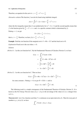
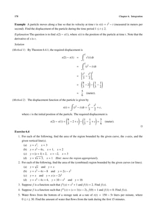
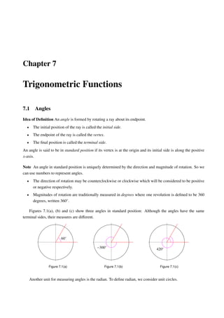
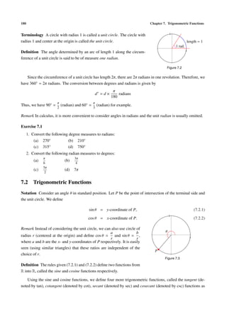
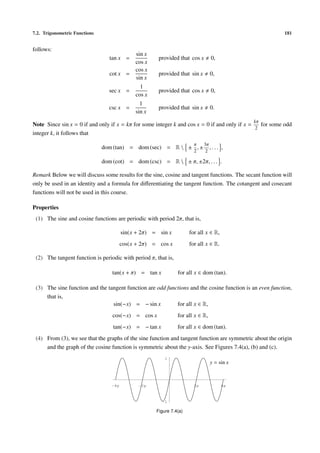
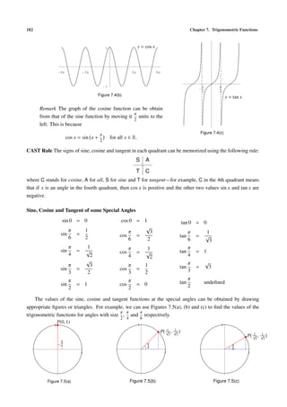
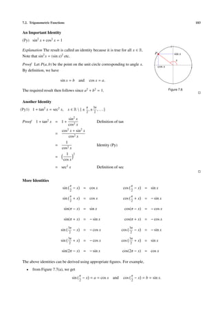
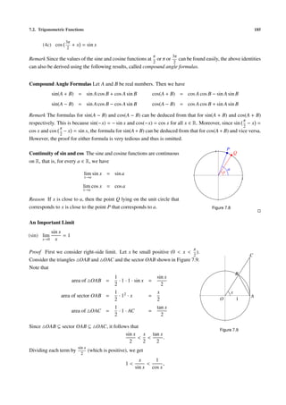
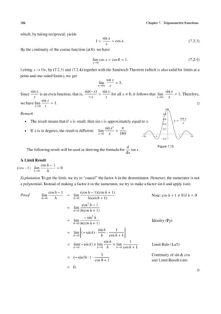
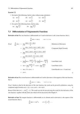
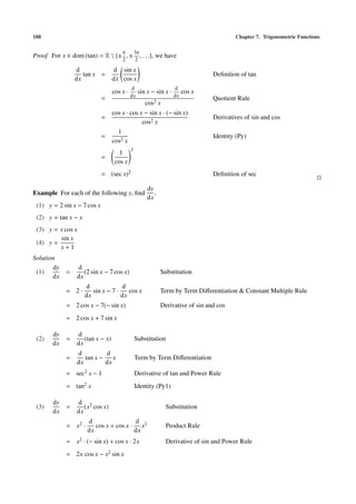
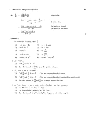
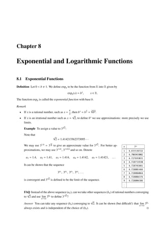
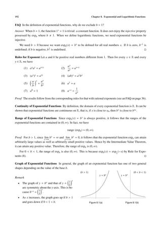
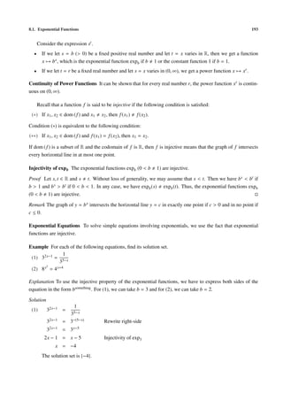
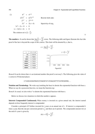
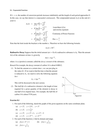
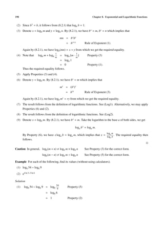
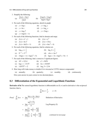
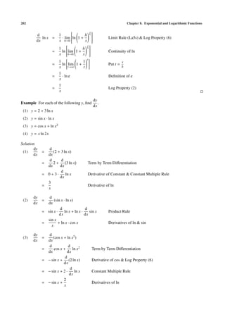
![206 Chapter 8. Exponential and Logarithmic Functions
Proof Put y = tan−1 x. Then we have x = tan y. From these we get
d dy
tan−1 x = Substitution
dx dx
1
= dx
Inverse Function Rule
dy
1
= d
Substitution
tan y
dy
1
= Derivative of tan
sec2 y
1
= Identity (Py1)
1 + tan2 y
1
= Substitution
1 + x2
Exercise 8.3
dy
1. For each of the following y, find .
dx
(a) y = 2x3 − 4e x − 5 (b) y = ln x − 1
(c) y = e x + ln x (d) y = x2 + ln x2
√ √
(e) y = ex + x (f) y = ln x − 1
(g) y = e x sin x (h) y = cos x ln x
(i) y = (x2 + 1)e x (j) y = (x2 + 1) ln x
ex ln x
(k) y= (l) y=
cos x sin x
x3 + 3x2 + 6x − 2 x3 + 3x2 + 6x − 2
(m) y= (n) y=
ex ln x
2. For each of the following f , find f (a) for the given a.
(a) f (x) = e x tan x, a = 0
ln x
(b) f (x) = , a=1
x2 + 1
d2 y
3. For each of the following f , find .
dx2
(a) y = x2 + x − 1 − e x
1
(b) y = 1 − ln x −
x
4. Use the inverse function rule to prove the following:
d 1
(a) sin−1 x = √ , −1 < x < 1
dx 1 − x2
d 1
(b) cos−1 x = −√ , −1 < x < 1
dx 1 − x2
π π
Note: The functions sin−1 and cos−1 are the inverses of the injective functions sin : − , −→ [−1, 1]
2 2
and cos : [0, π] −→ [−1, 1] respectively.](https://image.slidesharecdn.com/basiccalculus-120628005326-phpapp02/85/Basic-calculus-214-320.jpg)
![208 Chapter 9. More Differentiation
dy ∆y
= lim
dx ∆x→0 ∆x
∆y ∆u
= lim · Assume ∆u 0
∆x→0 ∆u ∆x
∆y ∆u
= lim · lim Limit Rule (L.5)
∆x→0 ∆u ∆x→0 ∆x
∆y ∆u
= lim · lim Continuity of f
∆u→0 ∆u ∆x→0 ∆x
dy du
= ·
du dx
d 2
Example Find (x + 5)3
dx
(1) without using chain rule;
(2) using chain rule.
Solution
d 2 d 6
(1) (x + 5)3 = (x + 15x4 + 75x2 + 125) Rewrite the function
dx dx
= 6x5 + 15 · 4x3 + 75 · 2x + 0 Term by Term Differentiation,
Constant Multiple Rule & Power Rule
= 6x5 + 60x3 + 150x
(2) Put u = x2 + 5 and put y = u3 . Then we have y = (x2 + 5)3 . From these we get
d 2 dy
(x + 5)3 = Substitution
dx dx
dy du
= · Chain Rule
du dx
d 3 d 2
= u · (x + 5) Substitution
du dx
= 3u2 · (2x + 0) Power Rule and Term by Term Differentiation
= 3(x2 + 5)2 · 2x Substitution
= 6x (x2 + 5)2
Remark
• It is straightforward to check that the above two results are the same.
1
• If we change the function to (x2 + 5) 3 , we can’t apply the first method but can still apply the second
method which makes use of the chain rule together with the power rule.
We can combine the chain rule with any formula to get a more general formula. In the table below, the gen-
eral form gives the derivative of g ◦ f where g is a power function, the sine function etc. and f is a differentiable
function such that g ◦ f is defined (for example, in order that ln[ f (x)] be defined, we have to assume that f is](https://image.slidesharecdn.com/basiccalculus-120628005326-phpapp02/85/Basic-calculus-216-320.jpg)
![9.1. Chain rule 209
positive). These formulas will be referred as the Chain Rule & Power Rule, Chain Rule & Derivative of sin etc.
1
For the Power Rule, we have seen that it is true if r is an integer or a rational number in the form n + where n
2
is an integer. In fact, it is true for all real numbers r. We will prove this result (called the General Power Rule)
later using logarithmic differentiation which is based on the Chain Rule & Derivative of ln.
Simple Form General Form
d r d d
x = rxr−1 [ f (x)]r = r[ f (x)]r−1 · f (x)
dx dx dx
d d d
sin x = cos x sin[ f (x)] = cos[ f (x)] · f (x)
dx dx dx
d d d
cos x = − sin x cos[ f (x)] = − sin[ f (x)] · f (x)
dx dx dx
d d d
tan x = sec2 x tan[ f (x)] = sec2 [ f (x)] · f (x)
dx dx dx
d x d f (x) d
e = ex e = e f (x) · f (x)
dx dx dx
d 1 d 1 d
ln x = ln[ f (x)] = · f (x)
dx x dx f (x) dx
Proof We give the proof for the 1st, 2nd and 6th formulas. The proofs of the rest are left as exercises.
(1) Put u = f (x) and put y = ur . Then we have y = [ f (x)]r . From these we get
d dy
[ f (x)]r = Substitution
dx dx
dy du
= · Chain Rule
du dx
d r du
= u · Substitution
du dx
du
= rur−1 · Power Rule
dx
d
= r[ f (x)]r−1 · f (x) Substitution
dx
(2) Put u = f (x) and put y = sin u. Then we have y = sin[ f (x)]. From these we get
d dy
sin[ f (x)] = Substitution
dx dx
dy du
= · Chain Rule
du dx
d du
= sin u · Substitution
du dx
du
= cos u · Derivative of sin
dx
d
= cos[ f (x)] · f (x) Substitution
dx](https://image.slidesharecdn.com/basiccalculus-120628005326-phpapp02/85/Basic-calculus-217-320.jpg)
![210 Chapter 9. More Differentiation
(6) Put u = f (x) and put y = ln u. Then we have y = ln[ f (x)]. From these we get
d dy
ln[ f (x)] = Substitution
dx dx
dy du
= · Chain Rule
du dx
d du
= ln u · Substitution
du dx
1 du
= · Derivative of ln
u dx
1 d
= · f (x) Substitution
f (x) dx
dy
Example For each of the following y, find .
dx
(1) y = sin(x2 + 1)
2 +2
(2) y = e x
(3) y = ln(x2 − 3)
2 +tan x2
(4) y = e x
(5) y = ln[sin2 (2x + 3)]
1
(6) y = 2
(x + 3)4
(7) y = e x+1 ln(x2 + 1)
Solution
dy d
(1) = sin(x2 + 1)
dx dx
d 2
= cos(x2 + 1) · (x + 1) Chain Rule & Derivative of sin
dx
= 2x cos(x2 + 1) Term by Term Differentiation and Power Rule
dy d x2 +2
(2) = e
dx dx
2 +2 d 2
= ex · (x + 2) Chain Rule & Derivative of exp
dx
2 +2
= 2x e x Term by Term Differentiation and Power Rule
dy d
(3) = ln(x2 − 3)
dx dx
1 d
= · (x2 − 3) Chain Rule & Derivative of ln
x2 − 3 dx
2x
= 2−3
Term by Term Differentiation and Power Rule
x](https://image.slidesharecdn.com/basiccalculus-120628005326-phpapp02/85/Basic-calculus-218-320.jpg)
![9.1. Chain rule 211
dy d x2 +tan x2
(4) = e
dx dx
2 +tan x2 d 2
= ex · (x + tan x2 ) Chain Rule & Derivative of exp
dx
2 +tan x2 d 2 d
= ex · x + tan x2 Term by Term Differentiation
dx dx
2 +tan x2 d 2
= ex · 2x + sec2 x2 · x Power Rule and Chain Rule & Derivative of tan
dx
2 +tan x2
= ex · (2x + sec2 x2 · 2x) Power Rule
2 +tan x2
= 2x (1 + sec2 x2 ) e x
dy d
(5) = ln[sin2 (2x + 3)]
dx dx
1 d
= 2
sin2 (2x + 3)
· Chain Rule & Derivative of ln
sin (2x + 3) dx
1 d
= 2
[sin(2x + 3)]2
· Rewrite sin2 u as (sin u)2
sin (2x + 3) dx
1 d
= 2
· 2 sin(2x + 3) · sin(2x + 3) Chain Rule & Power Rule
sin (2x + 3) dx
1 d
= 2
· 2 sin(2x + 3) · cos(2x + 3) · (2x + 3) Chain Rule & Derivative of sin
sin (2x + 3) dx
4 cos(2x + 3) Term by Term Differentiation
=
sin(2x + 3) and Power Rule
Remark In the above solution, we apply the chain rule thrice. Alternatively, we may use a property of
logarithm and apply the chain rule twice.
Alternative solution
dy d
= ln[sin2 (2x + 3)]
dx dx
d
= ln[sin(2x + 3)]2 Rewrite the function
dx
d
= 2 ln[sin(2x + 3)] Log Property (6)
dx
d
= 2· ln[sin(2x + 3)] Constant Multiple Rule
dx
1 d
= 2· · sin(2x + 3) Chain Rule & Derivative of ln
sin(2x + 3) dx
2 d
= · cos(2x + 3) · (2x + 3) Chain Rule & Derivative of sin
sin(2x + 3) dx
4 cos(2x + 3) Term by Term Differentiation
=
sin(2x + 3) and Power Rule](https://image.slidesharecdn.com/basiccalculus-120628005326-phpapp02/85/Basic-calculus-219-320.jpg)
![214 Chapter 9. More Differentiation
2 +cos x
(Step 1) Put y = 5 x .
(Step 2) Taking natural logarithm, we get
ln y = (x2 + cos x) ln 5.
(Step 3) Differentiating both sides with respect to x, we get
d d 2
ln y = (x + cos x) ln 5
dx dx
Chain Rule & Derivative of ln,
1 dy
· = ln 5 · (2x − sin x) Constant Multiple Rule, Term by Term Differentiation,
y dx
Power Rule and Derivative of cos
dy
= y (2x − sin x) ln 5
dx
2 +cos x
= (2x − sin x) 5 x ln 5 Substitution
Exercise 9.1
dy
1. Find for the following:
dx
√
(a) y = (2x3 + 5x2 )6 (b) y = 9 + 4x
√
4x2 + 5
(c) y= (d) y = cos 5x
3
(e) y = sin(6x − 7) (f) y = sin4 x
(g) y = cos5 (6x − 7) (h) y = 4x sin 3x
tan x
(i) y = tan(8x3 + 1) (j) y=
x+2
2
(k) y = 2e3x + 4x − 5 (l) y = x ex
x2
(m) y= (n) y = ln 8x
ex
(o) y = ln(5 − 2x) (p) y = ln(1 − x2 )
√
(q) y = ln 2x + 11 (r) y = 3x ln x
2
(s) y = ln(ln x) (t) y = e x ln x
(u) y = etan x (v) y = tan(e x )
(w) y = sin(e5x ) (x) y = esin 5x
(y) y = cos[ln(4x2 + 9)] (z) y = ln[cos(4x2 + 9)]
dy
2. Use logarithmic differentiation to find for the following:
dx
(a) y=2 x2 +1 (b) y = xx
(2x + 1)(3x + 4)5
(c) y = (sin x)cos x (d) y=
(x2 + 7)8
3. Ecologists estimate that when the population of a certain city is x thousand persons, the average level L of
carbon monoxide in the air above the city will be L ppm (parts per million), where L = 10+0.4x+0.001x2 .
The population of the city is estimated to be x = 345 + 22t + 0.5t2 thousand persons t years from the
present.
(a) Find the rate of change of carbon monoxide with respect to the population of the city.
(b) Find the time rate of change of the population when t = 3.
(c) How fast (with respect to time) is the carbon monoxide level changing at time t = 3?](https://image.slidesharecdn.com/basiccalculus-120628005326-phpapp02/85/Basic-calculus-222-320.jpg)
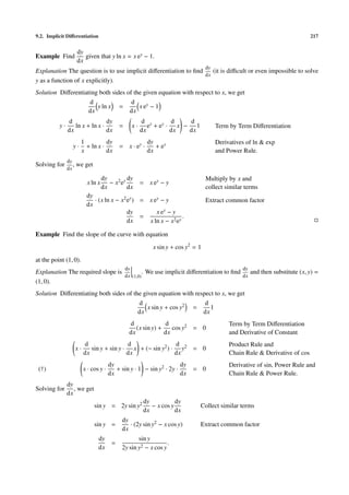
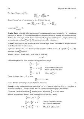
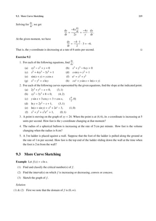
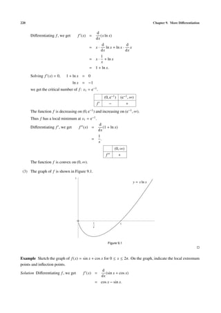
![9.3. More Curve Sketching 221
Solving f (x) = 0, cos x = sin x
tan x = 1
π 5π
we get the critical number of f in the interval (0, 2π): x1 = and x2 = .
4 4
π π 5π 5π
0, , , 2π
4 4 4 4
f + − +
π π 5π 5π
The function f is increasing on 0, , decreasing on , and increasing on , 2π .
4 4 4 4
π π π √ 5π 5π 5π √
Thus , f ( ) = , 2 is a local maximum point and , f( ) = , − 2 is a local minimum point of
4 4 4 4 4 4
the graph.
d
Differentiating f , we get f (x) = (cos x − sin x)
dx
= − sin x − cos x.
Solving f (x) = 0 in the interval [0, 2π]
− cos x = sin x
−1 = tan x
3π 7π
we get the zeros of f in the interval (0, 2π): x3 = and x4 = 4 .
4
3π 3π 7π 7π
0, , , 2π
4 4 4 4
f − + −
3π 3π 7π 7π
The function f is concave on 0, , convex on , and concave on , 2π .
4 4 4 4
3π 3π 3π 7π 7π 7π
Thus , f( ) = ,0 and , f( ) = ,0 are inflection points of the graph of f .
4 4 4 4 4 4
1
y = sin x + cos x
Π 3Π 5Π 7Π
4 4 4 4
1
Figure 9.2
Remark
• Because the sine and cosine functions are periodic with period 2π, we can use the above graph to get the
whole graph of f .](https://image.slidesharecdn.com/basiccalculus-120628005326-phpapp02/85/Basic-calculus-229-320.jpg)
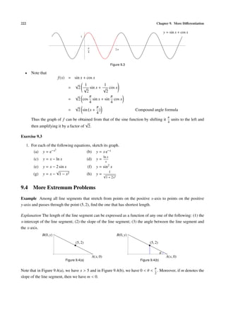
![9.4. More Extremum Problems 223
Solution 1 Let A(x, 0) and B(0, y) be the points of intersection of the line segment with the x- and y-axes
respectively. We want to minimize the length
L= x 2 + y2 .
Since the line segment passes through (5, 2), we get the following relationship between x and y.
y−2 2−0
=
0−5 5−x
−10
y = +2
5−x
2x
=
x−5
2
2x
Therefore, we have L = x2 + .
x−5
Since L is a minimum when L2 is a minimum, we consider minimizing
4x2
f (x) = x2 + , x > 5.
(x − 5)2
Differentiating, we get
d d
(x − 5)2 · (4x2 ) − 4x2 · (x − 5)2
dx dx
f (x) = 2x + 2
(x − 5)2
(x − 5)2 · 8x − 4x2 · 2(x − 5)
= 2x +
(x − 5)4
8x (x − 5) − 8x2
= 2x +
(x − 5)3
−40x
= 2x + .
(x − 5)3
40x
Solving f (x) = 0, 2x =
(x − 5)3
(x − 5)3 = 20 since x > 5 implies x 0
1
x − 5 = 20 3
√
3
we get the critical number of f in (5, ∞): x1 = 5 + 20.
√3 √
3
(5, 5 + 20) (5 + 20, ∞) 2x (x − 5)3 − 40x 2x [(x − 5)3 − 20]
Note that f (x) = = .
(x − 5)3 (x − 5)3
f − +
√3 √
3
Since f is decreasing on (5, 5 + 20) and increasing on (5 + 20, ∞), it follows that f attains its absolute
√
3
minimum at x1 . Therefore, the shortest line segment is the one that has x-intercept equal to (5 + 20, 0).
Solution 2 Let A(x, 0) and B(0, y) be the points of intersection of the line segment with the x- and y-axes
respectively. We want to minimize the length
L= x 2 + y2 .](https://image.slidesharecdn.com/basiccalculus-120628005326-phpapp02/85/Basic-calculus-231-320.jpg)
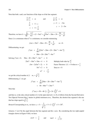
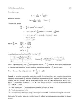
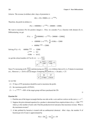

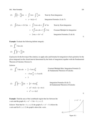
![232 Chapter 10. More Integration
The required area A is
0 2
A = [0 − (e x − 1)] dx + [(e x − 1) − 0] dx
−1 0
0 2
= (1 − e x ) dx + (e x − 1) dx
−1 0
Term by Term Integration,
0 2
= x − ex + ex − x Integration Formulas (1) & (6)
−1 0
& Fundamental Theorem of Calculus
= [(−1 + 0) − (−e−1 − 1)] + [(e2 − 2) − (1 − 0)]
= e2 + e−1 − 3
Exercise 10.1
1. Perform the following integration:
(a) 3 sec2 x dx (b) (2e x + cos x) dx
2x + 3 1 2
(c) dx (d) 1+ dx
x x
2. Evaluate the following definite integrals:
π
1
(a) 0
3
2 sin x dx (b) −1
(2e x + sin x) dx
−1 1 2 2−x
(c) −4
ex + dx (d) 1
dx
x x
3. Find the area of the (combined) region that
(a) lies between the x-axis and the graph of y = sin x for 0 ≤ x ≤ π;
1 1
(b) lies between the x-axis and the graph of y = for ≤ x ≤ e;
x 2
(c) lies under the graphs of y = e x and e−x and above the x-axis for −1 ≤ x ≤ 2 .
10.2 Substitution Method
Up to this stage, we can do simple integration using formulas and simple rules. For more complicated ones, like
2
x e x dx, we have to use some techniques for integration. In general, different forms of the integrand requires
different techniques. In this section, we discuss a simple but important technique — the substitution method. It
is the technique in integration that corresponds to the chain rule in differentiation.
Let y = F(u) be a function of u and let u = g(x) be a function of x. Then y can be considered as a function
of x by taking the composition of F with g:
y = F g(x) .
Suppose that the function g is differentiable on an open interval I and that the function F is differentiable on
an open interval containing the image of I under g. Then by the Chain Rule, the composition function F ◦ g is
differentiable on I and we have
d dy
F g(x) = Definition
dx dx
dy du
= · Chain Rule
du dx
= F (u) · g (x).](https://image.slidesharecdn.com/basiccalculus-120628005326-phpapp02/85/Basic-calculus-240-320.jpg)
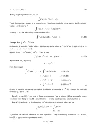
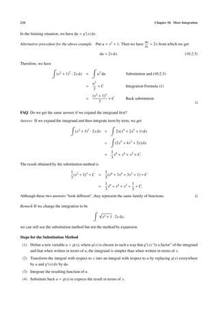
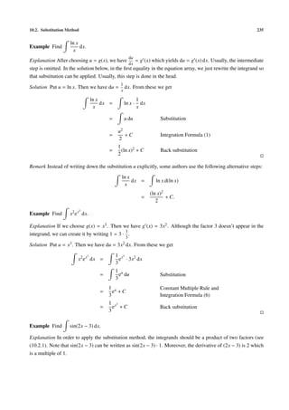
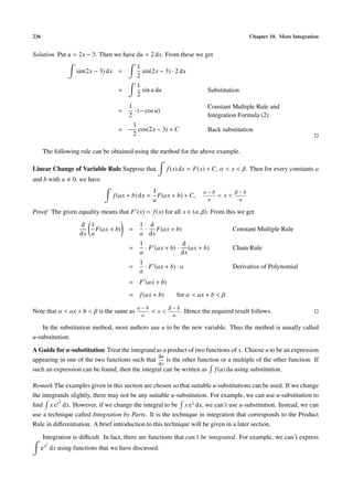
![10.2. Substitution Method 237
Substitution Method for Definite Integrals
To find definite integrals using u-substitution, one method is to find antiderivatives for the integrands and then
apply the Fundamental Theorem of Calculus. Alternatively, we may change of the definite integrals to ones in
terms of u by changing the limits of integration accordingly:
b g(b)
f g(x) g (x) dx = f (u) du (10.2.4)
a g(a)
where g is a continuous function on [a, b] and f is a function defined and continuous on an open interval I
containing the image of [a, b] under g.
Proof Let F be a function such that F = f on I. Note that F ◦ g is a primitive for ( f ◦ g) · g on [a, b]. Thus
we have
b b
f g(x) g (x) dx = F g(x) Fundamental Theorem of Calculus
a a
= F g(b) − F g(a)
g(b)
= F(u)
g(a)
g(b)
= f (u) du Fundamental Theorem of Calculus
g(a)
4
Example Evaluate x x2 + 9 dx.
0
Solution 1 Put u = x2 + 9. Then we have du = 2x dx. From these we get
1
x x2 + 9 dx = x2 + 9 · 2x dx
2
1 1
= u 2 du
2
3
1 u2
= · +C
2 32
1 2 3
= (x + 9) 2 + C.
3
By the Fundamental Theorem of Calculus, we have
4 4
1 2 3
x x2 + 9 dx = (x + 9) 2
0 3 0
1 1
= · 125 − · 27
3 3
98
=
3
Solution 2 Put u = x2 + 9. Then we have du = 2x dx.
Note that when x = 4, u = 25 and when x = 0, u = 9.](https://image.slidesharecdn.com/basiccalculus-120628005326-phpapp02/85/Basic-calculus-245-320.jpg)
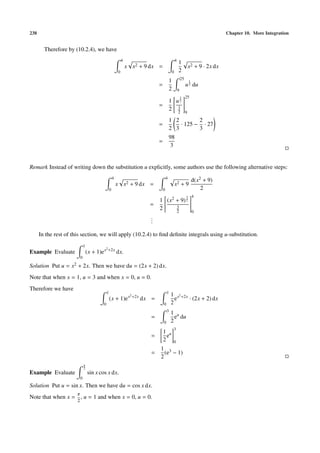
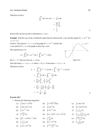
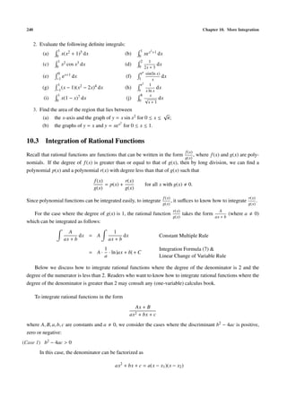
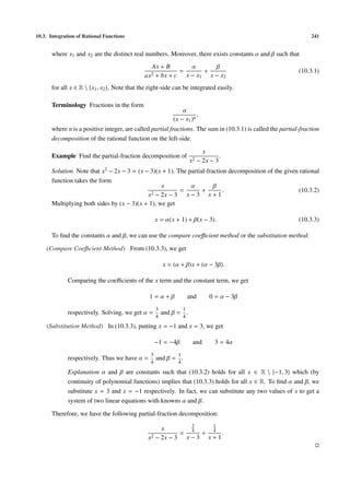
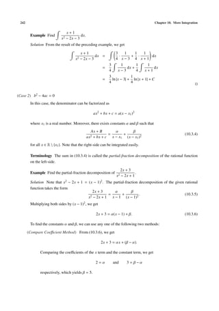
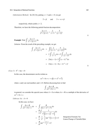
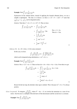
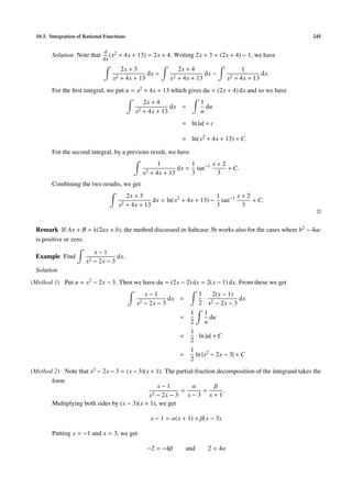
![10.5. More Applications of Definite Integrals 249
Note that (q0 , p0 ) is the intersection point of the demand curve and the supply curve.
The consumers’ surplus (denoted by CS ) and producers’ surplus (denoted by PS ) under market equilibrium
are defined as follows:
q0 q0
CS = [D(q) − p0 ] dq, PS = [p0 − S (q)] dq.
0 0
CS
PS
Figure 10.4(a) Figure 10.4(b)
Example Find the consumers’ surplus and producers’ surplus if the demand and supply equations are
q q2
p = D(q) = 20 − , p = S (q) = 2 + .
20 5000
Solution First we find the intersection point (q0 , p0 ) of the demand curve p = D(q) and the supply curve
p = S (q). Solving D(q) = S (q) (noting that q > 0)
q q2
20 − = 2+ (q > 0)
20 5000
q2 q
+ − 18 = 0 (q > 0)
5000 20
q2 + 250q − 90000 = 0 (q > 0)
(q − 200)(q + 450) = 0 (q > 0)
we get q0 = 200 and so p0 = D(200) = 10.
The consumers’ surplus is
200
CS = [D(q) − 10] dq
0
200
q
= 20 − − 10 dq
0 20
200
q
= 10 − dq
0 20
200
q2
= 10q −
40 0
= 1000.](https://image.slidesharecdn.com/basiccalculus-120628005326-phpapp02/85/Basic-calculus-257-320.jpg)
![250 Chapter 10. More Integration
The producers’ surplus is
200
PS = [10 − S (q)] dq
0
200
q2
= 10 − 2 + dq
0 5000
200
q2
= 8− dq
0 5000
200
q3
= 8q −
15000 0
3200
= .
3
Probability
To consider probabilities, the simplest method is to count, that is, to do addition. This works for the case
where the sample space is finite. However, if the sample space is infinite, we can’t count. To define probabilities,
we use definite integration which can be considered as a generalization of addition. Below we give a very brief
introduction to probabilities of events for continuous random variables.
Definition A variable whose values depend on the outcome of a random process is called a random variable.
Example
(1) Suppose a die is rolled and X1 is the number that turns up. Then X1 is a random variable with values in
{1, 2, 3, 4, 5, 6}.
(2) The life (in months) of a certain computer part is a random variable X2 with values in [0, ∞).
Note that the values that X1 can take are discrete whereas X2 can take any value in the interval [0, ∞). For this
we say that X1 is a discrete random variable and X2 a continuous random variable.
Definition Let X be a discrete random variable with values in {x1 , x2 , . . . , xn }. A probability function of X is a
function f with domain {x1 , x2 , . . . , xn } such that
(1) 0 ≤ f (xi ) for all i = 1, . . . , n;
(2) f (x1 ) + · · · + f (xn ) = 1.
Example Suppose a die is rolled and X is the number that turns up. If the die is fair, then the probability of
1
getting any one of the six numbers is . Thus we have the following probability function of X:
6
1
f (i) = for 1 ≤ i ≤ 6.
6
More generally, if the die is not fair, then the probability function g of X is given by
g(i) = wi for 1 ≤ i ≤ 6,
where 0 < wi < 1 and w1 + · · · + w6 = 1.](https://image.slidesharecdn.com/basiccalculus-120628005326-phpapp02/85/Basic-calculus-258-320.jpg)
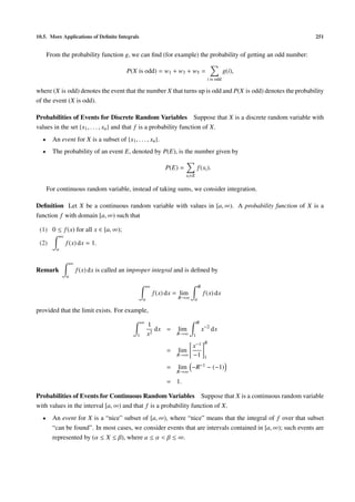
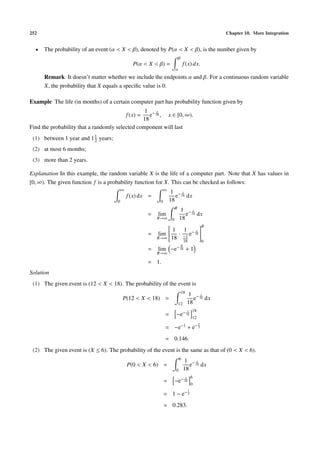
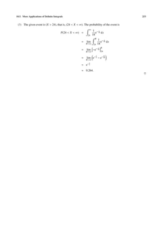

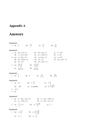
![256 Appendix A. Answers
Exercise 0.7
1. (a) 3x + 2y = 0 (b) 2x − y − 11 = 0 (c) 3x + y − 7 = 0
(d) 2x − y + 8 = 0 (e) 3x − y + 1 = 0 (f) y+1=0
Exercise 0.8
√ √
1. (a) 5 (b) 65 (c) 13 (d) 5 5
√
√ 3
2. (a) r = 3 C = (0, 2) (b) r = 3 C = (−2, 1) (c) r= C = (−1, 1 )
2
2
1 2
3. (a) 2 (b) √ (c) √
2 5
Exercise 0.9
1. (a) x-intercepts: (−6, 0), (2, 0), y-intercept: (0, −12), vertex: (−2, −16)
√
(b) x-intercepts: (3 ± 2, 0), y-intercept: (0, −7), vertex: (3, 2)
(c) no x-intercept, y-intercept: (0, 7), vertex: (− 1 , 13 )
2 2
Exercise 0.10
1. 8 cm × 6 cm
Exercise 1.1
1. (a) {2, 3, 5, 7}
(b) {2, 4, 6, 8, 10}
(c) {2}
(d) {1, 2, 3, 4, 5, 6, 7, 8, 9, 10, 11, 13, 17, 19}
(e) {1, 2, 3, 4, 5, 6, 7, 8, 9, 10, 12, 14, 16, 18}
(f) {2, 3, 4, 5, 6, 7, 8, 10, 11, 12, 13, 14, 16, 17, 18, 19}
(g) {1, 2, 3, 4, 5, 6, 7, 8, 9, 10, 11, 12, 13, 14, 16, 17, 18, 19}
(h) {2}
(i) {2, 4, 6, 8, 10}
(j) {2, 3, 4, 5, 6, 7, 8, 10, 12, 14, 16, 18}
(k) {1, 4, 6, 8, 9, 10}
(l) {12, 14, 15, 16, 18}
2. (a) False (b) False (c) True
Exercise 1.2
√ √ √
1. (a) { 2, − 2} (b) { 2} (c) ∅
2. (a) [3, 5] (b) [1, 9) (c) (1, 5)
(d) {5} (e) {1} (f) [3, 5) ∪ (5, 9)
(g) {5} (h) [1, ∞) (i) {5}
Exercise 1.3
7 29
1. (a) x ≤ − (b) x<−
5 3
7 5
(c) x>2 (d) x ≤ − or x ≥
2 11
√ √
3 − 41 3 + 41
(e) −1 < x < 3 (f) x< or x >
4 4
3
(g) no solution (h) x ≤ − or x > 4
2
(i) −7 < x < 4](https://image.slidesharecdn.com/basiccalculus-120628005326-phpapp02/85/Basic-calculus-264-320.jpg)
![257
2. (a) x(x + 5)(2x − 3) (b) (x − 1)(x + 1)(2x + 3)
(c) (x − 2)(x2 + x + 1) (d) x(x − 5)(x − 1)(x + 3)
(e) (x − 2)(x + 1)(x − 1)2 (f) (x − 1)2 (x2 + x + 2)
3 9
3. (a) − <x< or x > 4 (b) x≤3
2 5
3
(c) x < −2 or 1 < x < 3 (d) −3 ≤ x ≤ or x ≥ 2
2
(e) x>3 (f) x ≤ −1
5 3
(g) x < −4 or −2 < x < 1 or x > 3 (h) − ≤x≤
3 2
Exercise 2.1
3 6 a−4
1. (a) − (b) − (c)
8 65 a2 + 2a + 5
√
a−5 a2 − 5 a−5 4
(d) (e) (f) −
a+4 a4 + 4 a2 + 4 5
1 2 3
2. (a) (b) (c) √
2 3 4 2
1 √ (a2 + 1)|a|
(d) 1− + a (e)
a a2 + 2
3. (a) a2 + 2ab + b2 − 3a − 3b + 4 (b) −1 + h
(c) 2a − 3 + h
Exercise 2.2
√ √
1. (a) R (b) R { −6 }
5 (c) R {− 5, 5}
3
(d) R {−1, 3} (e) ( 2 , ∞) (f) [−3, ∞) { 1 }
2
(g) [− 5 , ∞) {−1, 1}
2 (h) (−∞, −5) ∪ (2, ∞)
2. (a) [−5, ∞) (b) [−4, ∞) (c) R {0}
(d) R {3} (e) (0, ∞) (f) (−∞, − 1 ] ∪ (0, ∞)
5
(g) (−∞, − 1 ] ∪ (0, ∞)
4
3. A(w) = 14w − w2 , dom = (0, 14), range = (0, 49]
Exercise 2.3
√ √ 2 2
1. x-intercept: ( 2, 0), (− 2, 0), y-intercept: 0, √ , (0, − √
3 3
2. a = 1, b = 1, c = −6
3. (a) y-intercept: (0, 5), no x-intercept
2 11
4. (a) (2, −1), 5, 5 (b) (2, −1), 2 , 5
3 3
(c){(2, 1), (2, −1), (−2, 1), (−2, −1)}
√
5. a=± 3
Exercise 2.4
1. (a) (b)
4 5
2
2 4 6 8 10
5
1 2 3 4
10
2](https://image.slidesharecdn.com/basiccalculus-120628005326-phpapp02/85/Basic-calculus-265-320.jpg)
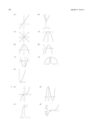
![262 Appendix A. Answers
cos x sin x
4. (a) x cos x + sin x (b) −
x + 1 (x + 1)2
2x (x2 + 1) cos x
(c) − (d) x(x + 2) cos x + 2(x + 1) sin x
sin x sin2 x
n−1 d
5. (c) n f (x) f (x)
dx
6. (a) 2(3x2 + 10x)(x3 + 5x2 − 2) (b) 6x(x2 + 5)2
Exercise 4.3
3 −1 1 3
1. (a) 6x − 6 (b) −4 (c) x 2 − x− 2
4 4
(d) 6x−4 − 4x−3 (e) 6x(5x3 + 2)
2. (a) 50 (b) −22 (c) 18
3. (a) a0 , a1 (b) an n(n − 1) · · · 1, 0
Exercise 5.1
1. (a) [ 5 , ∞)
4 (b) [−1, 1]
√ √
(c) (−∞, −7], [3, ∞) (d) (−∞, −3− 13 ], [ −3+ 13 , ∞)
2 2
(e) [−2, −1], [2, ∞) (f) (−∞, −2], [2, ∞)
7
2. (a) (local maximizer)
2
3
(b) 0 (neither), (local minimizer)
2
(c) −3 (local maximizer), 0 (neither), 3 (local minimizer)
(d) −2 (local maximizer), 0 (local minimizer)
3. (a) none (b) (2, ∞)
4
(c) 0, 5 , (1, ∞) (d) (0, ∞)
3
4. (a) − (b) 3
2
5. (a) (b)
40 10
20
1 1 2 3
2 2 4 6 10
20
20
(c) 20
(d) 10
15 5
10
5 2 1 1 2
5
3 2 1 1 2 3
Exercise 5.2
1. (a) minimum: −10, maximum: 82
(b) minimum: 0, maximum: 58
17
(c) minimum: −4, maximum:
16
2. 25, 25
3. x = 6, y = 3
4. 10 units by 10 units](https://image.slidesharecdn.com/basiccalculus-120628005326-phpapp02/85/Basic-calculus-270-320.jpg)
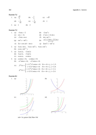
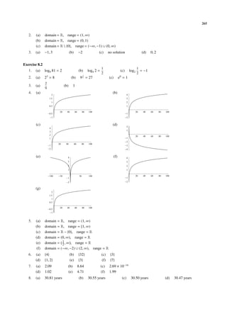
![266 Appendix A. Answers
Exercise 8.3
1
1. (a) 6x2 − 4e x (b)
x
1 2
(c) ex + (d) 2x +
x x
1 1
(e) ex + √ (f)
2 x 2x
cos x
(g) e x (sin x + cos x) (h) − sin x ln x
x
1
(i) (x + 1)2 e x (j) x + + 2x ln x
x
sin x − x ln x cos x
(k) (sin x + cos x)e x sec2 x (l)
x sin2 x
3x(x2 + 2x + 2) ln x − x3 − 3x2 − 6x + 2
(m) (8 − x3 )e−x (n)
x(ln x)2
1
2. (a) 1 (b)
2
1 2
3. (a) 2 − ex (b) 2
− 3
x x
Exercise 9.1
2
1. (a) 12x11 (2x + 5)5 (3x + 5) (b) √
9 + 4x
4x
(c) √ (d) −5 sin 5x
3 4x2 + 5
(e) 6 cos(6x − 7) (f) 4 sin3 x cos x
(g) −30 cos4 (6x − 7) sin(6x − 7) (h) 12x cos 3x + 4 sin 3x
sec2 x tan x
(i) 24x2 sec2 (8x3 + 1) (j) −
x+2 (x + 2)2
2
(k) 6e3x + 4 (l) (1 + 2x2 )e x
2x − x2 1
(m) (n)
ex x
−2 −2x
(o) (p)
5 − 2x 1 − x2
1
(q) (r) 3 + 3 ln x
2x + 11
2
1 ex 2
(s) (t) + 2xe x ln x
x ln x x
(u) etan x sec2 x (v) e x sec2 (e x )
(w) 5e5x cos(e5x ) (x) 5esin 5x cos 5x
−8x sin[ln(4x2 + 9)]
(y) (z) −8x tan(4x2 + 9)
4x2 + 9
2
2. (a) 2 x +2 x ln 2
(b) x x (1 + ln x)
(c) (sin x)cos x−1 cos2 x − (sin x)cos x+1 ln(sin x)
−16x(2x + 1)(3x + 4)5 15(2x + 1)(3x + 4)4 2(3x + 4)5
(d) + + 2
(x2 + 7)9 (x2 + 7)8 (x + 7)8
3. (a) 0.4 + 0.002x ppm/thousand
(b) 25 thousand/year
(c) 30.8 ppm/year
4. (a) 24](https://image.slidesharecdn.com/basiccalculus-120628005326-phpapp02/85/Basic-calculus-274-320.jpg)
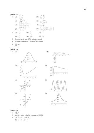
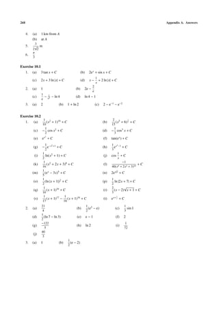
![270 Appendix B. Supplementary Notes
Then we have
k(k + 1)
1 + 2 + 3 + · · · + k + (k + 1) = + (k + 1) By (B.1.2)
2
k(k + 1) + 2(k + 1)
=
2
(k + 1)(k + 2)
=
2
(k + 1)[(k + 1) + 1]
=
2
that is, P(k + 1) is true.
Thus by the Principle of Mathematical Induction, P(n) is true for all positive integers n.
Example Use mathematical induction to show that the following is true for all positive integers n:
n(n + 1)(2n + 1)
12 + 22 + 32 + · · · + n2 = . (B.1.3)
6
Proof Denote (B.1.3) by P(n).
(I) When n = 1, we have
(1)(2)(3)
L.S . = 1 and R.S . = = 1.
6
Therefore P(1) is true.
(II) Suppose that P(k) is true, that is,
k(k + 1)(2k + 1)
12 + 22 + 32 + · · · + k2 = . (B.1.4)
6
Then we have
k(k + 1)(2k + 1)
12 + 22 + 32 + · · · + k2 + (k + 1)2 = + (k + 1)2 By (B.1.4)
6
k(k + 1)(2k + 1) + 6(k + 1)2
=
6
(k + 1)[k(2k + 1) + 6(k + 1)]
=
6
(k + 1)(2k2 + 7k + 6)
=
6
(k + 1)(k + 2)(2k + 3)
=
6
(k + 1)[(k + 1) + 1][(2(k + 1) + 1]
=
6
that is, P(k + 1) is true.
Thus by the Principle of Mathematical Induction, P(n) is true for all positive integers n.
Example Use mathematical induction (together with the product rule) to prove the power rule for positive
integers n:
d n
x = nxn−1 (B.1.5)
dx
Proof Denote (B.1.5) by P(n).](https://image.slidesharecdn.com/basiccalculus-120628005326-phpapp02/85/Basic-calculus-278-320.jpg)
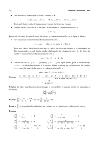
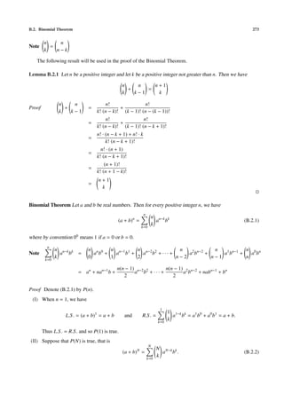
![274 Appendix B. Supplementary Notes
Then we have
(a + b)N+1 = (a + b)N · (a + b)
N
N N−k k
= (a + b) a b By B.2.2
k=0
k
N N
N N−k+1 k N N−k k+1
= a b + a b
k=0
k k=0
k
N N+1
N N−k+1 k N Replace k by k − 1 and
= a b + aN−(k−1) b(k−1)+1
k=0
k k=1
k−1 shift summation index
N
N N
= aN+1 + + aN−k+1 bk + bN+1
k=1
k k−1
N
N + 1 N−k+1 k
= aN+1 + a b + bN+1 By Lemma B.2.1
k=1
k
N+1
N + 1 N+1−k k
= a b
k=0
k
That is, P(N + 1) is true.
Hence by the Principle of Mathematical Induction, P(n) is true for all positive integers n.
B.3 Mean Value Theorem
Mean Value Theorem Let f be a function that is continuous on [a, b] and differentiable on (a, b), where
a, b ∈ R and a < b. Then there exists ξ ∈ (a, b) such that
f (b) − f (a)
f (ξ) = .
b−a
Explanation The conclusion means that there always exists (at least) a point C = ξ, f (ξ) on the graph of f ,
between A = a, f (a) and B = b, f (b) , such that the slope at C equals to the slope of the line AB.
Before giving the proof for the Mean Value Theorem, we prove a special case of the result.
Rolle’s Theorem Let g be a function that is continuous on [a, b] and differentiable on (a, b), where a, b ∈ R
and a < b. Suppose that g(a) = g(b). Then there exists ξ ∈ (a, b) such that
g (ξ) = 0.](https://image.slidesharecdn.com/basiccalculus-120628005326-phpapp02/85/Basic-calculus-282-320.jpg)
![B.3. Mean Value Theorem 275
Proof We may assume that g(a) = g(b) = 0; otherwise, we can replace g by g1 where g1 (x) = g(x) − g(a).
(Case 1) g is identically zero on [a, b]
In this case, g (x) = 0 for all x ∈ (a, b). So any ξ ∈ (a, b) satisfies the requirement.
(Case 2) g is not identically zero on [a, b]
By the Extreme Value Theorem, g attains its maximum and minimum in [a, b], that is, there exists ξ1 and
ξ2 in [a, b] such that
g(ξ1 ) ≤ g(x) ≤ g(ξ2 ) for all x ∈ [a, b].
Since g is not identically zero on [a, b], it follows that at least one of ξ1 , ξ2 is not an endpoint of [a, b].
Hence there exists ξ ∈ (a, b) such that g has a local maximum or minimum at ξ. Therefore, by Theo-
rem 5.1.3, we have g (ξ) = 0.
Proof of the Mean Value Theorem Instead of working on f , we construct an auxiliary function g so that Rolle’s
Theorem can be applied to g and the conclusion for g is what we want for f .
Let g : [a, b] −→ R be the function defined by
f (b) − f (a)
g(x) = f (x) − f (a) − (x − a) for x ∈ [a, b].
b−a
Note that g is continuous on [a, b] and differentiable on (a, b) with
f (b) − f (a)
g (x) = f (x) − for x ∈ (a, b).
b−a
Moreover, we have g(b) = g(a) = 0. Hence by Rolle’s Theorem, there exists ξ ∈ (a, b) such that g (ξ) = 0, or
equivalently that
f (b) − f (a)
f (ξ) = .
b−a
Remark If f is a function that is differentiable on an open interval I, then for every x1 , x2 ∈ I with x1 < x2 , the
function f is continuous on [x1 , x2 ] and differentiable on (x1 , x2 ) and so we can apply the Mean Value Theorem
to f with a = x1 and b = x2 .
Below we apply the Mean Value to prove the following result which is Theorem 5.1.1.
Theorem B.3.1 Let f be a function that is defined and differentiable on an open interval (a, b).
(1) If f (x) > 0 for all x ∈ (a, b), then f is increasing on (a, b).
(2) If f (x) < 0 for all x ∈ (a, b), then f is decreasing on (a, b).](https://image.slidesharecdn.com/basiccalculus-120628005326-phpapp02/85/Basic-calculus-283-320.jpg)
![276 Appendix B. Supplementary Notes
(3) If f (x) = 0 for all x ∈ (a, b), then f is constant on (a, b), that is, f (x1 ) = f (x2 ) for all x1 , x2 ∈ (a, b), or
equivalently, there exists a real number c such that f (x) = c for all x ∈ (a, b).
Proof We give the proof for (1) and (3). The proof for (2) is similar to that for (1). Alternatively, to prove (2),
we may apply (1) to the function − f .
(1) Suppose that f (x) > 0 for all x ∈ (a, b). Let x1 , x2 ∈ (a, b) where x1 < x2 . By the Mean Value Theorem,
there exists ξ ∈ (x1 , x2 ) ⊆ (a, b) such that
f (x2 ) − f (x1 )
f (ξ) = .
x2 − x1
Therefore, we have
f (x2 ) − f (x1 ) = (x2 − x1 ) f (ξ) > 0,
which implies that f (x1 ) < f (x2 ).
(3) Suppose that f (x) = 0 for all x ∈ (a, b). From the proof of (1), we see that for every pair of x1 , x2 in
(a, b), there exists ξ ∈ (a, b) such that
f (x2 ) − f (x1 ) = (x2 − x1 ) f (ξ) = 0.
which implies that f (x1 ) = f (x2 ). Thus f is a constant function.
B.4 Fundamental Theorem of Calculus
Before giving the proof of the Fundamental Theorem of Calculus (Version 1), we need some preliminary results.
Lemma B.4.1 Let f and g be functions that are continuous on a closed and bounded interval [a, b]. Suppose
that f (x) ≤ g(x) for all x ∈ [a, b]. Then we have
b b
f (x) dx ≤ g(x) dx.
a a
Proof By definition, we have
b n
b−a i
(g − f )(x) dx = lim (g − f )(xi−1 ) · , where xi = a + (b − a) for 0 ≤ i ≤ n.
a n→∞ n n
i=1
The condition on f and g implies that each term in the above sum is non-negative. Hence we have
b
(g − f )(x) dx ≥ 0.
a
The required inequality then follows from Rules for Definite Integral (Int1) and (Int2).
Corollary B.4.2 Let f be a function that is continuous on a closed and bounded interval [a, b]. Suppose that m
and M are real numbers such that m ≤ f (x) ≤ M for all x ∈ [a, b]. Then we have
b
m(b − a) ≤ f (x) dx ≤ M(b − a).
a](https://image.slidesharecdn.com/basiccalculus-120628005326-phpapp02/85/Basic-calculus-284-320.jpg)
![B.4. Fundamental Theorem of Calculus 277
Proof By Lemma B.4.1, we have
b b b
m dx ≤ f (x) dx ≤ M dx.
a a a
The required inequalities then follow from Definite Integral for Constant.
The next result is known as the Mean Value Theorem for Definite Integral.
Theorem B.4.3 Let f be a function that is continuous on a closed and bounded interval [a, b]. Then there
exists ξ ∈ [a, b] such that
b
f (x) dx = f (ξ) · (b − a).
a
Proof By the Extreme Value Theorem, there exist x1 , x2 ∈ [a, b] such that
f (x1 ) ≤ f (x) ≤ f (x2 ) for all x ∈ [a, b].
By considering the constant functions f (x1 ) and f (x2 ) on the interval [a, b] and applying Corollary B.4.2, we
get
b
f (x1 ) · (b − a) ≤ f (x) dx ≤ f (x2 ) · (b − a),
a
which yields
b
a
f (x) dx
f (x1 ) ≤≤ f (x2 ).
b−a
By the Intermediate Value Theorem, there exists ξ between x1 and x2 such that
b
a
f (x) dx
f (ξ) = .
b−a
Hence the required result follows.
Fundamental Theorem of Calculus, Version 1 Let f be a function that is continuous on a closed and bounded
interval [a, b]. Let F be the function from [a, b] into R defined by
x
F(x) = f (t) dt for a ≤ t ≤ b.
a
Then F is continuous on [a, b] and differentiable on (a, b) with F (x) = f (x) for all x ∈ (a, b).
Proof We divide the proof into two parts: continuity and differentiability.
(Continuity) By the Extreme Value Theorem, there exist real numbers m and M such that
m ≤ f (x) ≤ M for all x ∈ [a, b]. (B.4.1)
Let x1 , x2 ∈ [a, b] with x1 < x2 . By the construction of F together with Rule for Definite Integral (Int3),
we have x x x
1 2 1
F(x2 ) − F(x1 ) = f (t) dt + f (t) dt − f (t) dt
a x1 a
x2
= f (t) dt
x1](https://image.slidesharecdn.com/basiccalculus-120628005326-phpapp02/85/Basic-calculus-285-320.jpg)
![278 Appendix B. Supplementary Notes
which, by (B.4.1) and Corollary B.4.2, yields
m(x2 − x1 ) ≤ F(x2 ) − F(x1 ) ≤ M(x2 − x1 ). (B.4.2)
For every α ∈ (a, b), putting x1 = α and x2 = x, by (B.4.2) and the Sandwich Theorem, we see that
lim F(x) − F(α) = 0,
x→α+
that is, lim F(x) = F(α); similarly putting x2 = α and x1 = x, we see that
x→α+
lim F(x) = F(α);
x→α−
hence we have lim F(x) = F(α), that is, F is continuous at α. Similarly, the function F is left-continuous
x→α
at a and right-continuous at b. Therefore F is continuous on [a, b].
(Differentiability) Let x ∈ (a, b). We want to show that
F(x + h) − F(x)
lim = f (x).
h→0 h
For this, we consider left-side and right-side limits.
For h > 0, by the construction of F together with Rule for Definite Integral (Int3), we have
x+h
F(x + h) − F(x) = f (t) dt.
x
Hence by Theorem B.4.3, there exists ξh ∈ [x, x + h] such that
F(x + h) − F(x) = f (ξh ) · (x + h) − x = f (ξh ) · h.
Note that as h tends to 0 from the right, the number ξh tends to x (from the right). Therefore, we have
F(x + h) − F(x)
lim = lim f (ξh ) = f (x) (B.4.3)
h→0+ h h→0+
by the continuity of f .
For h < 0, by the construction of F together with Rule for Definite Integral (Int3), we have
x
F(x) − F(x + h) = f (t) dt.
x+h
Hence by Theorem B.4.3, there exists ξh ∈ [x + h, x] such that
F(x) − F(x + h) = f (ξh ) · x − (x + h) = f (ξh ) · (−h).
Note that as h tends to 0 from the left, the number ξh tends to x (from the left). Therefore, we have
F(x + h) − F(x)
lim = lim f (ξh ) = f (x) (B.4.4)
h→0− h h→0−
by the continuity of f .
Combining (B.4.3) and (B.4.4), we get
F(x + h) − F(x)
lim = f (x)
h→0 h
as required.
Remark Rule for Definite Integral (Int3) can be proved using a property of continuous functions on closed and
bounded interval, namely, uniform continuity. This concept is discussed in more advanced calculus or analysis.](https://image.slidesharecdn.com/basiccalculus-120628005326-phpapp02/85/Basic-calculus-286-320.jpg)


![[Sundstrom_Ted.]_Mathematical_Reasoning_Writing - Copy.pdf](https://cdn.slidesharecdn.com/ss_thumbnails/sundstromted-221124155318-3b41c59e-thumbnail.jpg?width=640&height=640&fit=bounds)


![Getting Started with Apache Spark: Big Data Made Simple [Free Meetup]](https://cdn.slidesharecdn.com/ss_thumbnails/apachesparkgettingstarted-260203175547-8361bcc3-thumbnail.jpg?width=640&height=640&fit=bounds)
