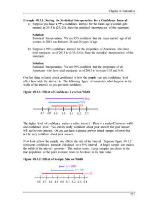
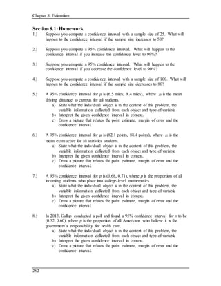
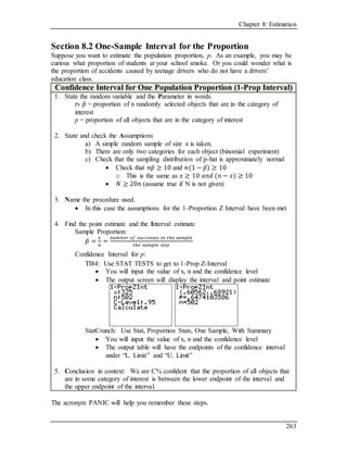
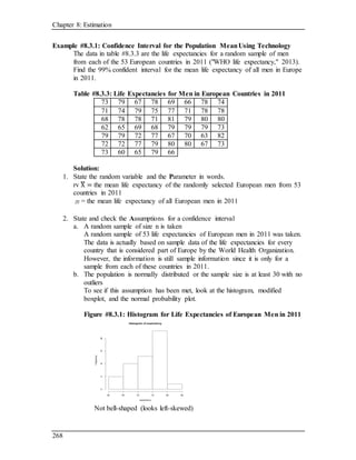
This document discusses confidence intervals for estimating population parameters. It provides examples of constructing point and interval estimates for the population mean and proportion from sample data. Confidence intervals allow us to estimate a range of plausible values for the true population parameter based on the sample results and desired confidence level, rather than just a single point value. The width of the confidence interval depends on the sample size and confidence level, with larger samples and lower confidence levels producing narrower intervals.
1. Chapter 8: Estimation
260
Chapter 8: Estimation
In hypothesis tests, the purpose was to make a decision about a population parameter, in
terms of it being greater than, less than, or not equal to a claimed value. But what if you
want to actually know what the value of the parameter is. You need to do estimation.
There are two types of estimation – point estimates and interval estimates (confidence
intervals).
Section 8.1 Basics of Confidence Intervals
Point estimate – a single number computed from sample data used to estimate a
parameter value
A point estimate is just the statistic that you have calculated previously.
When we have qualitative data, we are going to use 𝑝̂ as a point estimate for p
When we have quantitative data, we are going to use 𝑥̅ as a point estimate for 𝜇
Larger samples tend to give us better point estimates since the distribution of possible
values of a random variable is less spread out for larger sample sizes. But it would be
rare for our sample result to match the population parameter value perfectly. So, instead
of looking at a single number, the point estimate, we look at an entire interval of plausible
values for the parameter called an interval estimate.
Interval estimate (confidence interval) – an interval of numbers around the point
estimate that we will have a certain level of confidence contains the true value of the
population parameter.
In general, a confidence interval when using a symmetric distribution looks like the
following: point estimate ± margin of error.
point estimate – margin of error point estimate point estimate + margin of error
(---------------------------*---------------------------)
⏟
interval estimate
Interpreting a confidence interval:
If you could actually take every sample of size n from a given population and compute
the corresponding point estimate and C% confidence interval for the parameter from each
set of sample data, 𝐶% of those intervals would actually contain the true value of the
parameter and (100 − 𝐶)% of the intervals would not. Unfortunately, we do not get to
take every sample of size n from a given population. We usually get one sample which
will yield one point estimate and one interval estimate. We will never know if the
interval we computed actually contains the true value of the parameter or not. All we can
say is that we are 𝐶% confident that it does. Be careful not to use the word “chance” or
“probability” with a given confidence interval. These are words that we use when talking
about random variables (because these values vary from one sample to another). In this
section we are talking about parameters. These values are some fixed value (we just
don’t know what that fixed value is).
2. Chapter 8: Estimation
261
Example #8.1.1: Stating the Statistical Interpretation for a Confidence Interval
a) Suppose you have a 95% confidence interval for the mean age a woman gets
married in 2013 is (26, 28). State the statistical interpretation of this statement.
Solution:
Statistical Interpretation: We are 95% confident that the mean marital age of all
women in 2013 was between 26 and 28 years of age.
b) Suppose a 99% confidence interval for the proportion of Americans who have
tried marijuana as of 2013 is (0.35, 0.41). State the statistical interpretation of this
statement.
Solution:
Statistical Interpretation: We are 99% confident that the proportion of all
Americans who have tried marijuana as of 2013 is between 0.35 and 0.41.
One last thing to know about confidence is how the sample size and confidence level
affect how wide the interval is. The following figure demonstrates what happens to the
width of the interval as you get more confident.
Figure #8.1.1: Effect of Confidence Level on Width
The higher level of confidence makes a wider interval. There’s a tradeoff between width
and confidence level. You can be really confident about your answer but your answer
will not be very precise. Or you can have a precise answer (small margin of error) but
not be very confident about your answer.
Now look at how the sample size affects the size of the interval. Suppose figure #8.1.2
represents confidence intervals calculated on a 95% interval. A larger sample size makes
the width of the interval narrower. This makes sense. Large samples are closer to the
true population so the point estimate tends to be closer to the true value.
Figure #8.1.2: Effect of Sample Size on Width
3. Chapter 8: Estimation
262
Section8.1:Homework
1.) Suppose you compute a confidence interval with a sample size of 25. What will
happen to the confidence interval if the sample size increases to 50?
2.) Suppose you compute a 95% confidence interval. What will happen to the
confidence interval if you increase the confidence level to 99%?
3.) Suppose you compute a 95% confidence interval. What will happen to the
confidence interval if you decrease the confidence level to 90%?
4.) Suppose you compute a confidence interval with a sample size of 100. What will
happen to the confidence interval if the sample size decreases to 80?
5.) A 95% confidence interval for 𝜇 is (6.5 miles, 8.4 miles), where m is the mean
driving distance to campus for all students.
a) State what the individual object is in the context of this problem, the
variable information collected from each object and type of variable
b) Interpret the given confidence interval in context.
c) Draw a picture that relates the point estimate, margin of error and the
confidence interval.
6.) A 95% confidence interval for 𝜇 is (82.1 points, 88.4 points), where m is the
mean exam score for all statistics students.
a) State what the individual object is in the context of this problem, the
variable information collected from each object and type of variable
b) Interpret the given confidence interval in context.
c) Draw a picture that relates the point estimate, margin of error and the
confidence interval.
7.) A 95% confidence interval for p is (0.68, 0.71), where p is the proportion of all
incoming students who place into college-level mathematics.
a) State what the individual object is in the context of this problem, the
variable information collected from each object and type of variable
b) Interpret the given confidence interval in context.
c) Draw a picture that relates the point estimate, margin of error and the
confidence interval.
8.) In 2013, Gallup conducted a poll and found a 95% confidence interval for p to be
(0.52, 0.60), where p is the proportion of all Americans who believe it is the
government’s responsibility for health care.
a) State what the individual object is in the context of this problem, the
variable information collected from each object and type of variable
b) Interpret the given confidence interval in context.
c) Draw a picture that relates the point estimate, margin of error and the
confidence interval.
4. Chapter 8: Estimation
263
Section 8.2 One-Sample Interval for the Proportion
Suppose you want to estimate the population proportion, p. As an example, you may be
curious what proportion of students at your school smoke. Or you could wonder what is
the proportion of accidents caused by teenage drivers who do not have a drivers’
education class.
Confidence Interval for One Population Proportion (1-Prop Interval)
1. State the random variable and the Parameter in words.
rv 𝑝̂ = proportion of n randomly selected objects that are in the category of
interest
p = proportion of all objects that are in the category of interest
2. State and check the Assumptions
a) A simple random sample of size n is taken.
b) There are only two categories for each object (binomial experiment)
c) Check that the sampling distribution of p-hat is approximately normal
Check that 𝑛𝑝̂ ≥ 10 and 𝑛(1 − 𝑝̂) ≥ 10
o This is the same as 𝑥 ≥ 10 𝑎𝑛𝑑 (𝑛 − 𝑥) ≥ 10
𝑁 ≥ 20𝑛 (assume true if N is not given)
3. Name the procedure used.
In this case the assumptions for the 1-Proportion Z Interval have been met
4. Find the point estimate and the Interval estimate
Sample Proportion:
𝑝̂ =
𝑥
𝑛
=
𝑛𝑢𝑚𝑏𝑒𝑟 𝑜𝑓 𝑠𝑢𝑐𝑐𝑒𝑠𝑠𝑒𝑠 𝑖𝑛 𝑡ℎ𝑒 𝑠𝑎𝑚𝑝𝑙𝑒
𝑡ℎ𝑒 𝑠𝑎𝑚𝑝𝑙𝑒 𝑠𝑖𝑧𝑒
Confidence Interval for p:
TI84: Use STAT TESTS to get to 1-Prop Z-Interval
You will input the value of x, n and the confidence level
The output screen will display the interval and point estimate
StatCrunch: Use Stat, Proportion Stats, One Sample, With Summary
You will input the value of x, n and the confidence level
The output table will have the endpoints of the confidence interval
under “L. Limit” and “U. Limit”
5. Conclusion in context: We are C% confident that the proportion of all objects that
are in some category of interest is between the lower endpoint of the interval and
the upper endpoint of the interval.
The acronym PANIC will help you remember these steps.
5. Chapter 8: Estimation
264
Example #8.2.1: Confidence Interval for the Population Proportion Using
Technology
A researcher studying the effects of income levels on breastfeeding of infants
hypothesizes that countries where the income level is lower have a higher rate of
infant breastfeeding than higher income countries. It is known that in Germany,
considered a high-income country by the World Bank, 22% of all babies are
breastfeed. In Tajikistan, considered a low-income country by the World Bank,
researchers found that in a random sample of 500 new mothers that 125 were
breastfeeding their infants. Find a 90% confidence interval of the proportion of
all mothers in Tajikistan who breastfeed their infants?
Solution:
1. State the random variable and the Parameter in words.
rv 𝑝̂ = proportion of 500 new mothers in Tajikistan who breastfeed
p = proportion of all new mothers in Tajikistan who breastfeed
2. State and check the Assumptions
a) A simple random sample of size n is taken.
A simple random sample of 500 new mothers from Tajikistan was
taken
b) There are only two categories for each object (binomial experiment)
Either a new mother from Tajikistan breastfeeds of she doesn’t
c) Check that the sampling distribution of 𝑝̂ is approximately normal
Check that 𝑥 ≥ 10 𝑎𝑛𝑑 (𝑛 − 𝑥) ≥ 10
𝑥 = 125 ≥ 10 and ( 𝑛 − 𝑥) = 500 − 125 = 375 ≥ 10
𝑁 ≥ 20𝑛 (assume true if N is not given)
No N is given so we will assume 𝑁 ≥ 20𝑛
3. Name the procedure used.
In this case the assumptions for the 1-Proportion Z Interval have been met
4. Find the point estimate and the confidence Interval
Sample Proportion:
𝑝̂ =
𝑥
𝑛
=
125
500
= 0.25
Confidence Interval for p:
TI-84: Go into STAT arrow over to TESTS and choose 1-PropZInt.
Input Output
5. Conclusion in context: We are 90% confident that the proportion of all new
mothers in Tajikistan who breastfeed their infants is between 0.218 and 0.282.
6. Chapter 8: Estimation
265
Or we could also say we are 90% confident that the percentage of all new mothers
in Tajikistan who breastfeed their infants is between 21.8% and 28.2%
Sometimes these intervals are reported as follows: We estimate that 25% of all
new mothers in Tajikistan breastfeed their infants (with a margin of error of about
3.2%)
25% - 3.2% 25% 25% + 3.2%
(---------------------------*---------------------------)
⏟
interval estimate for p
𝑝̂ ± 𝑀𝐸
25% ± 3.2%
7. Chapter 8: Estimation
266
Section8.2:Homework
In each problem show all steps of the confidence interval (PANIC). If some of the
assumptions are not met, note that the results of the interval may not be correct and then
continue the process of the confidence interval.
1.) It is believed that 11% of all Americans are left-handed. In a random sample of
200 students from a particular college with 10345 students, 30 were left-handed.
Find a 99% confidence interval for the percentage of all students at this particular
college who are left-handed.
2.) In November of 2013, Australians were asked if they thought unemployment
would increase. At that time 284 out of 631 said that they thought unemployment
would increase ("Morgan gallup poll," 2013). Estimate the proportion of all
Australians in November 2013 who believed unemployment would increase using
a 95% confidence interval.
3.) According to the February 2008 Federal Trade Commission report on consumer
fraud and identity theft, Arkansas had 1,601 complaints of identity theft out of
3,482 consumer complaints ("Consumer fraud and," 2008). Calculate a 90%
confidence interval for the proportion of all complaints that are complaints of
identity theft in Arkansas.
4.) According to the February 2008 Federal Trade Commission report on consumer
fraud and identity theft, Alaska had 321 complaints of identity theft out of 1,432
consumer complaints ("Consumer fraud and," 2008). Calculate a 90% confidence
interval for the proportion of all complaints that are complaints of identity theft in
Alaska.
5.) In 2013, the Gallup poll asked 1,039 American adults if they believe there was a
conspiracy in the assassination of President Kennedy, and found that 634 believe
there was a conspiracy ("Gallup news service," 2013). Estimate the proportion of
all American’s who believe in this conspiracy using a 98% confidence interval.
6.) In 2008, there were 507 children in Arizona out of 32,601 who were diagnosed
with Autism Spectrum Disorder (ASD) ("Autism and developmental," 2008).
Find the proportion of all children in Arizona diagnosed with ASD with a
confidence level of 99%.
8. Chapter 8: Estimation
267
Section 8.3 One-Sample Interval for the Mean
Suppose you want to estimate the mean height of all Americans, or you want to estimate
the mean salary of all college graduates. In these cases, we need a confidence interval for
the population mean.
Confidence Interval for One Population Mean (t-Interval)
1. State the random variable and the Parameter in words.
rv 𝑥̅ = the mean measurement of n randomly selected objects
m = the mean measurement of all objects
2. State and check the Assumptions for a hypothesis test
a. A random sample of size n is taken.
b. The population is normally distributed or the sample size is at least 30 with
no outliers
If you are given data, you can use the methods from 6.4
c. The population standard deviation, 𝜎, is unknown.
3. Name the procedure used
In this case the assumptions for the T Interval have been met
4. Find the point estimate and confidence Interval
Sample mean:
𝑥̅ =
∑ 𝑥
𝑛
, this value is given or you can get it from 1-Var Stats
Confidence interval for 𝜇:
TI84: Use STAT arrow over to TEST and choose T-Interval
Highlight “Data” if you entered a list of data or “Stats” if given stats
The output screen will have the interval and point estimate.
StatCrunch: Use Stat, T Stats, One Sample, With Data (or With Summary)
If you have data, then select the column and confidence level
If you have summary stats, fill in the sample mean, sample std dev,
sample size, and confidence level.
The output table will have the endpoints of the confidence interval
under “L. Limit” and “U. Limit”
5. Conclusion in context: We are C% confident that the mean measurement of all
objects is between the lower endpoint and the upper endpoint.
9. Chapter 8: Estimation
268
Example #8.3.1: Confidence Interval for the Population MeanUsing Technology
The data in table #8.3.3 are the life expectancies for a random sample of men
from each of the 53 European countries in 2011 ("WHO life expectancy," 2013).
Find the 99% confident interval for the mean life expectancy of all men in Europe
in 2011.
Table #8.3.3: Life Expectancies for Men in European Countries in 2011
73 79 67 78 69 66 78 74
71 74 79 75 77 71 78 78
68 78 78 71 81 79 80 80
62 65 69 68 79 79 79 73
79 79 72 77 67 70 63 82
72 72 77 79 80 80 67 73
73 60 65 79 66
Solution:
1. State the random variable and the Parameter in words.
rv X̅ = the mean life expectancy of the randomly selected European men from 53
countries in 2011
m = the mean life expectancy of all European men in 2011
2. State and check the Assumptions for a confidence interval
a. A random sample of size n is taken
A random sample of 53 life expectancies of European men in 2011 was taken.
The data is actually based on sample data of the life expectancies for every
country that is considered part of Europe by the World Health Organization.
However, the information is still sample information since it is only for a
sample from each of these countries in 2011.
b. The population is normally distributed or the sample size is at least 30 with no
outliers
To see if this assumption has been met, look at the histogram, modified
boxplot, and the normal probability plot.
Figure #8.3.1: Histogram for Life Expectancies of European Men in 2011
Not bell-shaped (looks left-skewed)
Histogram of expectancy
expectancy
Frequency
60 65 70 75 80 85
05101520
10. Chapter 8: Estimation
269
Figure #8.3.2: Modified Box Plot for Life Expectancies of European Men
in 2011
There are no outliers for this data set.
Figure #8.3.3: Normal Probability Plot for Life Expectancies of European
Menin 2011
Not linear
This population does not appear to be normally distributed. However, the sample
size is at least 30 and the modified boxplot showed no outliers.
3. Name the procedure used.
The conditions for the T Interval have been met.
60 65 70 75 80
Life Expectancies of European Men in 2011
Life Expectancies
-2 -1 0 1 2
6065707580
Normal Q-Q Plot
Theoretical Quantiles
SampleQuantiles
11. Chapter 8: Estimation
270
4. Find the point estimate and confidence Interval
TI-84: Go into the STAT menu, and type the data into L1.
Then go into STAT and over to TESTS. Choose TInterval.
Figure #8.3.4: Setup for TInterval
Figure #8.3.5: Results for TInterval
StatCrunch: Enter or upload the data into StatCrunch first.
Then go to Stat, T Stats, One Sample, With Data
Select the column of data to use and then enter the confidence level:
The output screen will have the point estimate (sample mean) and the endpoints
of the interval estimate (L. Limit and U. Limit).
No matter which technology you use you get the following:
Sample mean:
𝑥̅ ≈ 73.736 years
Confidence interval for 𝜇:
(71.632 years, 75.840 years)
12. Chapter 8: Estimation
271
5. Conclusion in context:
We are 99% confident that the mean life expectancy of all European men in 2011
was between 71.6 years and 75.8 years.
Sometimes these intervals are reported as follows: We estimate that the mean life
expectancy of all European men in 2011 is about 73.7 years (with a margin of
error of about 2.1 years)
73.7 – 2.1 73.7 73.7 + 2.1
(---------------------------*---------------------------)
⏟
interval estimate for 𝜇
X̅ ± 𝑀𝐸
73.7 𝑦𝑒𝑎𝑟𝑠 ± 2.1 𝑦𝑒𝑎𝑟𝑠
Section8.3:Homework
In each problem show all steps of the confidence interval (PANIC). If some of the
assumptions are not met, note that the results of the interval may not be correct and then
continue the process of the confidence interval.
1.) The Kyoto Protocol was signed in 1997, and required countries to start reducing
their carbon emissions. The protocol became enforceable in February 2005.
Table 8.3.4 contains CO2 emissions from a random sample of 30 countries in
2010 ("CO2 emissions," 2013). Compute a 99% confidence interval to estimate
the mean CO2 emission for all countries in 2010.
Table #8.3.4: CO2 Emissions (metric tons per capita) in 2010
1.36 1.42 5.93 5.36 0.06 9.11 7.32 2.86
7.93 6.72 0.78 1.80 0.20 2.27 0.28 2.44
5.86 3.46 1.46 0.14 2.62 0.79 7.48
0.86 7.84 2.87 2.45 5.85 3.45 1.45
2.) Many people feel that cereal is healthier alternative for children over glazed
donuts. Table #8.3.5 contains the amount of sugar in a random sample of cereal
that is geared towards children ("Healthy breakfast story," 2013). Estimate the
mean amount of sugar in all children’s cereals using a 95% confidence level.
Table #8.3.5: Sugar Amounts (g) in Children’s Cereal
10 14 12 9 13 13 13
11 12 15 9 10 11 3
6 12 15 12 12
13. Chapter 8: Estimation
272
3.) In Florida, bass fish were collected in 53 randomly selected lakes to measure the
amount of mercury in the fish. The data for the average amount of mercury in
each lake is in table #8.3.6 ("Multi-disciplinary niser activity," 2013). Compute a
90% confidence interval for the mean amount of mercury in fish in all Florida
lakes.
Table #8.3.6: Average Mercury Levels (mg/kg) in Fish
1.23 1.33 0.04 0.44 1.20 0.27
0.48 0.19 0.83 0.81 0.71 0.5
0.49 1.16 0.05 0.15 0.19 0.77
1.08 0.98 0.63 0.56 0.41 0.73
0.34 0.59 0.34 0.84 0.50 0.34
0.28 0.34 0.87 0.56 0.17 0.18
0.19 0.04 0.49 1.10 0.16 0.10
0.48 0.21 0.86 0.52 0.65 0.27
0.94 0.40 0.43 0.25 0.27
4.) In 1882, Albert Michelson collected measurements on the speed of light ("Student
t-distribution," 2013). His measurements are given in table #8.3.7. Find the speed
of light value that Michelson estimated from his data using a 95% confidence
interval.
Table #8.3.7: Speed of Light Measurements (km/sec)
299883 299816 299778 299796 299682
299711 299611 299599 300051 299781
299578 299796 299774 299820 299772
299696 299573 299748 299748 299797
299851 299809 299723
5.) Table #8.3.8 contains pulse rates after running for 1 minute, collected from a
random sample of 30 females who drink alcohol ("Pulse rates before," 2013).
Find a 95% confidence interval for the mean pulse rate after exercise of all
women who do drink alcohol.
Table #8.3.8: Pulse Rates (beats per minute) of Woman Who Use Alcohol
176 150 150 115 129 160
120 125 89 132 120 120
68 87 88 72 77 84
92 80 60 67 59 64
88 74 68 115 110 117
14. Chapter 8: Estimation
273
6.) The economic dynamism, which is the index of productive growth in dollars for
countries that are designated by the World Bank as middle-income, for a random
sample of 22 middle-income countries are in table #8.3.9 ("SOCR data 2008,"
2013). Compute a 95% confidence interval for the mean economic dynamism of
all middle-income countries.
Table #8.3.9: Economic Dynamism ($) of Middle-Income Countries
25.8057 37.4511 51.915 43.6952 47.8506 43.7178 58.0767
41.1648 38.0793 37.7251 39.6553 42.0265 48.6159 43.8555
49.1361 61.9281 41.9543 44.9346 46.0521 48.3652 43.6252
50.9866 59.1724 39.6282 33.6074 21.6643
7.) Table #8.3.10 contains the percentage of woman receiving prenatal care in 2009
for a sample of countries ("Pregnant woman receiving," 2013). Estimate the
mean percentage of woman receiving prenatal care in all countries in 2009 using a
90% confidence interval.
Table #8.3.10: Percentage of Woman Receiving Prenatal Care
100.0 72.73 74.52 75.79 76.28 76.28
76.65 80.34 80.60 81.90 86.30 87.70
87.76 88.40 90.70 91.50 91.80 92.10
92.20 92.41 92.47 93.00 93.20 93.40
93.63 93.68 93.80 94.30 94.51 95.00
95.80 95.80 96.23 96.24 97.30 97.90
97.95 98.20 99.00 99.00 99.10 99.10
100.00 100.00 100.00 100.00
8.) Maintaining your balance may get harder as you grow older. A study was
conducted to see how steady the elderly are on their feet. They had the subjects
stand on a force platform and have them react to a noise. The force platform then
measured how much they swayed forward and backward, and the data from a
sample of 9 elderly people is in table #8.3.11 ("Maintaining balance while,"
2013). Find a 99% confidence interval for the mean sway of all elderly people.
Table #8.3.11: Forward/backward Sway (mm) of Elderly Subjects
19 30 20 19 29 25 21 24 50
15. Chapter 8: Estimation
274
Data Sources:
Australian Human Rights Commission, (1996). Indigenous deaths in custody 1989 -
1996. Retrieved from website: http://www.humanrights.gov.au/publications/indigenous-
deaths-custody
CDC features - new data on autism spectrum disorders. (2013, November 26). Retrieved
from http://www.cdc.gov/features/countingautism/
CDC features - new data on autism spectrum disorders. (2013, November 26). Retrieved
from http://www.cdc.gov/features/countingautism/
Center for Disease Control and Prevention, Prevalence of Autism Spectrum Disorders -
Autism and Developmental Disabilities Monitoring Network. (2008). Autism and
developmental disabilities monitoring network-2012. Retrieved from website:
http://www.cdc.gov/ncbddd/autism/documents/ADDM-2012-Community-Report.pdf
CO2 emissions. (2013, November 19). Retrieved from
http://data.worldbank.org/indicator/EN.ATM.CO2E.PC
Federal Trade Commission, (2008). Consumer fraud and identity theft complaint data:
January-december 2007. Retrieved from website:
http://www.ftc.gov/opa/2008/02/fraud.pdf
Federal Trade Commission, (2008). Consumer fraud and identity theft complaint data:
January-december 2007. Retrieved from website:
http://www.ftc.gov/opa/2008/02/fraud.pdf
Gallup news service. (2013, November 7-10). Retrieved from
http://www.gallup.com/file/poll/165896/JFK_Conspiracy_131115.pdf
Gallup news service. (2013, November 7-10). Retrieved from
http://www.gallup.com/file/poll/165896/JFK_Conspiracy_131115.pdf
Healthy breakfast story. (2013, November 16). Retrieved from
http://lib.stat.cmu.edu/DASL/Stories/HealthyBreakfast.html
IQ of famous people. (2013, November 13). Retrieved from
http://www.kidsiqtestcenter.com/IQ-famous-people.html
Maintaining balance while concentrating. (2013, September 25). Retrieved from
http://www.statsci.org/data/general/balaconc.html
16. Chapter 8: Estimation
275
Morgan Gallup poll on unemployment. (2013, September 26). Retrieved from
http://www.statsci.org/data/oz/gallup.html
Morgan Gallup poll on unemployment. (2013, September 26). Retrieved from
http://www.statsci.org/data/oz/gallup.html
Multi-disciplinary niser activity - mercury in bass. (2013, November 16). Retrieved from
http://gozips.uakron.edu/~nmimoto/pages/datasets/MercuryInBass - description.txt
Pregnant woman receiving prenatal care. (2013, October 14). Retrieved from
http://data.worldbank.org/indicator/SH.STA.ANVC.ZS
Pulse rates before and after exercise. (2013, September 25). Retrieved from
http://www.statsci.org/data/oz/ms212.html
SOCR data 2008 world countries rankings. (2013, November 16). Retrieved from
http://wiki.stat.ucla.edu/socr/index.php/SOCR_Data_2008_World_CountriesRankings
Student t-distribution. (2013, November 25). Retrieved from
http://lib.stat.cmu.edu/DASL/Stories/student.html
WHO life expectancy. (2013, September 19). Retrieved from
http://www.who.int/gho/mortality_burden_disease/life_tables/situation_trends/en/index.h
tml