1
JADAVPUR UNIVERSITY
Authored by: DEBARATI ROY
2
HYPOTHESIS TESTING:-
Hypothesis testing is a statistical method that is used in making statistical decisions
using experimental data. Hypothesis Testing is basically an assumption that we make
about the population parameter.
WHY DO WE USE IT?
Hypothesis testing is an essential procedure in statistics. A hypothesis test evaluates
two mutually exclusive statements about a population to determine which statement
is best supported by the sample data. When we say that a finding is statistically
significant, it’s thanks to a hypothesis test.
WHAT ARE BASICS OF HYPOTHESIS ?
The basic of hypothesis is normalization and standard normalization. all our
hypothesis is revolve around basic of these 2 terms.
WHICH ARE IMPORTANT PARAMETERS OF HYPOTHESIS TESTING ?
Null hypothesis :- In inferential statistics, the null hypothesis is a general statement or
default position that there is no relationship between two measured phenomena, or
no association among groups.
WHAT IS HYPOTHESIS TESTING?
3
Alternative hypothesis :-The alternative hypothesis is the hypothesis used in hypothesis
testing that is contrary to the null hypothesis. It is usually taken to be that the observations
are the result of a real effect (with some amount of chance variation superposed).
Level of significance:- Refers to the degree of significance in which we accept or reject
the null-hypothesis. 100% accuracy is not possible for accepting or rejecting a
hypothesis, so we therefore select a level of significance that is usually 5%.
Type I error: When we reject the null hypothesis, although that hypothesis was true.
Type I error is denoted by alpha. In hypothesis testing, the normal curve that shows the
critical region is called the alpha region.
Type II errors: When we accept the null hypothesis but it is false. Type II errors are
denoted by beta. In Hypothesis testing, the normal curve that shows the acceptance
region is called the beta region.
One tailed test :- A test of a statistical hypothesis , where the region of rejection is on
only one side of the sampling distribution , is called a one-tailed test.
Two-tailed test :- A two-tailed test is a statistical test in which the critical area of a
distribution is two-sided and tests whether a sample is greater than or less than a certain
range of values. If the sample being tested falls into either of the critical areas, the
alternative hypothesis is accepted instead of the null hypothesis.
P-value :- The P value, or calculated probability, is the probability of finding the observed,
or more extreme, results when the null hypothesis (H 0) of a study question is true — the
definition of ‘extreme’ depends on how the hypothesis is being tested. If your P value is
less than the chosen significance level then you reject the null hypothesis i.e. accept that
your sample gives reasonable evidence to support the alternative hypothesis. It does NOT
imply a “meaningful” or “important” difference; that is for you to decide when
considering the real-world relevance of your result.
4
TYPES OF HYPOTHESIS TESTS
Univariate-Tests Multivariate-Tests
N=2 N>2
Parametric Non-parametric
Two-Samples Test More-Than-Two-samples (N=Number Of Samples)
PARAMETRIC UNIVARIATE TESTS(TWO-SAMPLES):-
1. Two-sample-T test(comparison of means)
2. Z-test(comparison of means)
3. Fisher-Exact-test(comparison of variances)
PARAMETRIC UNIVARIATE TESTS(MORE THAN TWO SAMPLES):-
1. ANOVA test
2. Bartlett’s test(comparison of variances)
NON-PARAMETRIC TESTS:-
1. McNemar Test(for two samples)
2. Chi-Square Test(two as well as more than two samples)
3. Median Test(for two or more than two samples)
4. Mann-Whitney Test
5
5. Two-Sample-Kolmogorov-Smrinov-test
MULTIVARIATE TESTS:-
1. Hotelling’s Multivariate T2
-Test(for two samples)
2. MANOVA Test(more than two samples)
TWO-SAMPLE-T –TEST:-
What is a Two-Sample T-Test?
A two-sample t-test is used when you want to compare two independent groups to
see if their means are different.
The Independent Samples t Test or 2-sample t-test compares the means of two
independent groups in order to determine whether there is statistical evidence
that the associated population means are significantly different. The
Independent Samples t Test is a parametric test. This test is also known as:
Independent t Test.
We have 2 fields, our objective is to compare the yield between on different samples.
(Using T value method)
t - value = (Signal/Noise) = (Difference between the means/variability of group)
Formula = |X1-X2|/Sqrt((S1^2/n1)+(S2^2/n2))
T test is applied when
1) population Standard deviation is not available.
2) n is less than 30.
6
(X1=mean of sample 1. X2=mean of sample 2. S1=variance of sample 1. S2=variance
of sample 2. n1=size of sample 1. n2= size of sample 2.)
Z-TEST:-
We would use a Z test if:
 Your sample size is greater than 30. Otherwise, use a t test.
 Data points should be independent from each other. In other words, one data
point isn’t related or doesn’t affect another data point.
 Your data should be normally distributed. However, for large sample sizes (over
30) this doesn’t always matter.
 Your data should be randomly selected from a population, where each item has
an equal chance of being selected.
 Sample sizes should be equal if at all possible.
The formula is same as Two-Sample-T-test.
FISHER-EXACT-TEST
The Fisher Exact test is a test of significance that is used in the place of chi square test
in 2 by 2 tables, especially in cases of small samples.
The Fisher Exact test tests the probability of getting a table that is as strong due to
the chance of sampling. The word ‘strong’ is defined as the proportion of the cases
that are diagonal with the most cases.
7
The Fisher Exact test is a test of significance that is used in the place of chi square test
in 2 by 2 tables, especially in cases of small samples.
There are certain terminologies that help in understanding the theory of Fisher Exact
test.
The Fisher Exact test uses the following formula:
p= ( ( a + b ) ! ( c + d ) ! ( a + c ) ! ( b + d ) ! ) / a ! b ! c ! d ! N !
In this formula, the ‘a,’ ‘b,’ ‘c’ and ‘d’ are the individual frequencies of the 2X2
contingency table, and ‘N’ is the total frequency.
The Fisher Exact test uses this formula to obtain the probability of the combination of
the frequencies that are actually obtained. It also involves the finding of the
probability of every possible combination which indicates more evidence of
association.
ANOVA TEST:-
The t-test works well when dealing with two groups, but sometimes we
want to compare more than two groups at the same time. For example, if we wanted
to test whether voter age differs based on some categorical variable like race, we have
to compare the means of each level or group the variable. We could carry out a
separate t-test for each pair of groups, but when you conduct many tests you increase
the chances of false positives. The analysis of variance or ANOVA is a statistical
inference test that lets you compare multiple groups at the same time.
F = Between group variability / Within group variability.
8
Unlike the z and t-distributions, the F-distribution does not have any negative values
because between and within-group variability are always positive due to squaring
each deviation.
One Way F-test(Anova) :- It tell whether two or more groups are similar or not based
on their mean similarity and f-score.
What does this test do?
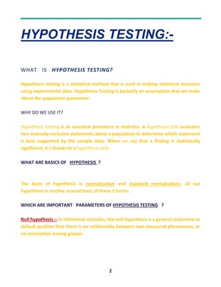
The one-way ANOVA compares the means between the groups you are interested in
and determines whether any of those means are statistically significantly different
from each other. Specifically, it tests the null hypothesis:
Where µ = group mean and k = number of groups. If, however, the one-way ANOVA
returns a statistically significant result, we accept the alternative hypothesis (HA),
which is that there are at least two group means that are statistically significantly
different from each other.
BARTLETT’S TEST
There are actually two tests called Bartlett’s. The first is for Bartlett’s test for
homogeneity of variances and the second is Bartlett’s test for sphericity (testing that
the correlation matrix has an identity matrix).
Bartlett’s test for homogeneity of variances is used to test that variances are equal
for all samples. It checks that the assumption of equal variances is true before
running certain statistical tests like the One-Way ANOVA. It’s used when you’re fairly
certain your data comes from a normal distribution.
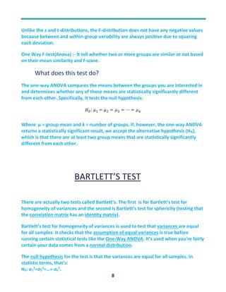
The null hypothesis for the test is that the variances are equal for all samples. In
statistic terms, that’s:
H0: σ1
2
=σ2
2
=…= σk
2
.
9
The alternate hypothesis (the one you’re testing), is that the variances are not equal
for one pair or more:
H0: σ1
2
≠ σ2
2
≠… ≠ σk
2
.
The test statistic is :
McNnmar’s TEST:-
The McNemar’s test operates upon a contingency table.
10
A contingency table is a tabulation or count of two categorical variables. In the case of
the McNemar’s test, we are interested in binary variables correct/incorrect or yes/no
for a control and a treatment or two cases. This is called a 2×2 contingency table.
The McNemar’s test is checking if the disagreements between two cases match.
Technically, this is referred to as the homogeneity of the contingency table (specifically
the marginal homogeneity). Therefore, the McNemar’s test is a type of homogeneity
test for contingency tables.
In terms of comparing two binary classification algorithms, the test is commenting on
whether the two models disagree in the same way (or not). It is not commenting on
whether one model is more or less accurate or error prone than another. This is clear
when we look at how the statistic is calculated.
The McNemar’s test statistic is calculated as:
statistic = (Yes/No - No/Yes)^2 / (Yes/No + No/Yes)
Where Yes/No is the count of test instances that Classifier1 got correct and Classifier2
got incorrect, and No/Yes is the count of test instances that Classifier1 got incorrect
and Classifier2 got correct.
CHI-SQUARE-TEST:-
11
The test is applied when you have two categorical variables from a single population.
It is used to determine whether there is a significant association between the two
variables.
In research, there are studies which often collect data on categorical variables that
can be summarized as a series of counts. These counts are commonly arranged in a
tabular format known as a contingency table. The chi-square test statistic can be used
to evaluate whether there is an association between the rows and columns in a
contingency table. More specifically, this statistic can be used to determine whether
there is any difference between the study groups in the proportions of the risk factor
of interest. Chi-square test and the logic of hypothesis testing were developed by Karl
Pearson.
Chi-square test is a nonparametric test used for two specific purpose: (a) To test the
hypothesis of no association between two or more groups, population or criteria (i.e.
to check independence between two variables); (b) and to test how likely the observed
distribution of data fits with the distribution that is expected (i.e., to test the
goodness-of-fit). It is used to analyze categorical data (e.g. male or female patients,
smokers and non-smokers, etc.), it is not meant to analyze parametric or continuous
data (e.g., height measured in centimeters or weight measured in kg, etc.).
 This test only works for categorical data (data in categories), such as Gender {Men,
Women} or color {Red, Yellow, Green, Blue} etc, but not numerical data such as height
or weight.
 The numbers must be large enough. Each entry must be 5 or more.
Chi-Square Formula
This is the formula for Chi-Square:
 O = the Observed (actual) value
 E = the Expected value.
12
MEDIAN-TEST
The median test is a non-parametric test that is used to test
whether two (or more) independent groups differ in central tendency - specifically
whether the groups have been drawn from a population with the same median. The
null hypothesis is that the groups are drawn from populations with the same median.
The alternative hypothesis can be either that the two medians are different (two-
tailed test) or that one median is greater than the other (one-tailed test).
The principle of the test is that if two samples have the same median, they should have
more or less the same proportion of observations above and below that median. This
would be true irrespective of their two distributions. If any scores fall at the value of
the combined median they may either be dropped from the analysis, or included with
scores less than the median.
The median test is a special case of the chi-square test for independence. Given k
samples with n1, n2, ..., nk observations, compute the grand median of all n1 + n2 + ... + nk
observations. Then construct a 2xk contingency table where row one contains the
number of observations above the grand median for each of the k samples and row two
contains the number of observations below or equal to the grand median for each of the
k samples. The chi-square test for independence can then be applied to this table. More
specifically
H0: All k populations have the same median
Ha: All least two of the populations have different medians
13
The advantage of median test over Mann Whitney is that it only tests for differences
in the median irrespective of any differences in the shape of the distribution.
MANN-WHITNEY TEST
Mann-Whitney U test is the non-parametric alternative test to the
independent sample t-test. It is a non-parametric test that is used to compare two
sample means that come from the same population, and used to test whether two
sample means are equal or not. Usually, the Mann-Whitney U test is used when the
data is ordinal or when the assumptions of the t-test are not met.
Mann-Whitney U test is a non-parametric test, so it does not assume any assumptions
related to the distribution of scores. There are, however, some assumptions that are
assumed
1. The sample drawn from the population is random.
2. Independence within the samples and mutual independence is assumed. That means
that an observation is in one group or the other (it cannot be in both).
3. Ordinal measurement scale is assumed.
HOTELLING’S-MULTIVARIATE-T2-TEST:-
Hotelling’s T-Squared (Hotelling, 1931) is the multivariate
counterpart of the T-test. “Multivariate” means that you have data for more than one
parameter for each sample. For example, let’s say you wanted to compare how well two
different sets of students performed in school. You could compare univariate data (e.g.
14
mean test scores) with a t-test. Or, you could use Hotelling’s T-squared to compare
multivariate data (e.g. the mutivariate mean of test scores, GPA, and class grades).
Hotelling’s T-Squared is based on Hotelling’s T2
distribution and forms the basis for
various multivariate.
Hotelling’s T-squared has several advantages over the t-test (Fang, 2017):
 The Type I error rate is well controlled,
 The relationship between multiple variables is taken into account,
 It can generate an overall conclusion even if multiple (single) t-tests are
inconsistent. While a t-test will tell you which variable differ between groups,
Hotelling’s summarizes the between-group differences.
The test hypotheses are:
 Null hypothesis (H0): the two samples are from populations with the same
multivariate mean.
 Alternate hypothesis (H1): the two samples are from populations with different
multivariate means.
Three major assumptions are that the samples:
 …have underlying normal distributions.
 …are independent.
 …have equal variance-covariance matrices (for the two sample test only). Run
Bartlett’s test to check this assumption.
Hotelling’s-T can be transformed to an F-statistic.
15
Like the t-test, you’ll want to find a value for T (in this case, for T-squared) and compare
it to a table value; if the calculated value is greater than the table statistic, you can reject
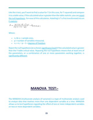
the null hypothesis. For ease of this calculation, Hotelling’s t2
is first transformed into an
F-statistic:
Where:
 n1 & n2 = sample sizes,
 p = number of variables measured,
 n1 + n2 – p – 1 = degrees of freedom.
Reject the null hypothesis (at a chosen significance level) if the calculated value is greater
than the F-table critical value. Rejecting the null hypothesis means that at least one of
the parameters, or a combination of one or more parameters working together, is
significantly different.
MANOVA TEST:-
The MANOVA (multivariate analysis of variance) is a type of multivariate analysis used
to analyze data that involves more than one dependent variable at a time. MANOVA
allows us to test hypotheses regarding the effect of one or more independent variables
on two or more dependent variables.
16
A MANOVA analysis generates a p-value that is used to determine whether or not the
null hypothesis can be rejected.
MANOVA provides a solution for some studies. This statistical procedure tests multiple
dependent variables at the same time. By doing so, MANOVA can offer several
advantages over ANOVA.
Comparison of MANOVA to ANOVA Using an Example
MANOVA can detect patterns between multiple dependent variables. But, what does
that mean exactly? Let’s work through an example that compares ANOVA to MANOVA.
Suppose we are studying three different classification methods of supervised machine
learning algorithm. This variable is our independent variable. We also have false-positive
values and true-positive values. These variables are our dependent variables. We want
to determine whether the mean scores for false-positive and true-positive differ
between the three teaching methods.
When MANOVA Provides Benefits
Use multivariate ANOVA when your dependent variables are correlated. The correlation
structure between the dependent variables provides additional information to the
model which gives MANOVA the following enhanced capabilities:
 Greater statistical power: When the dependent variables are correlated,
MANOVA can identify effects that are smaller than those that regular ANOVA
can find.
 Assess patterns between multiple dependent variables: The factors in the model
can affect the relationship between dependent variables instead of influencing
a single dependent variable. As the example in this post shows, ANOVA tests
with a single dependent variable can fail completely to detect these patterns.
 Limits the joint error rate: When you perform a series of ANOVA tests because
you have multiple dependent variables, the joint probability of rejecting a true
null hypothesis increases with each additional test. Instead, if you perform one
MANOVA test, the error rate equals the significance level.

Hypothesis

  • 1.
  • 2.
    2 HYPOTHESIS TESTING:- Hypothesis testingis a statistical method that is used in making statistical decisions using experimental data. Hypothesis Testing is basically an assumption that we make about the population parameter. WHY DO WE USE IT? Hypothesis testing is an essential procedure in statistics. A hypothesis test evaluates two mutually exclusive statements about a population to determine which statement is best supported by the sample data. When we say that a finding is statistically significant, it’s thanks to a hypothesis test. WHAT ARE BASICS OF HYPOTHESIS ? The basic of hypothesis is normalization and standard normalization. all our hypothesis is revolve around basic of these 2 terms. WHICH ARE IMPORTANT PARAMETERS OF HYPOTHESIS TESTING ? Null hypothesis :- In inferential statistics, the null hypothesis is a general statement or default position that there is no relationship between two measured phenomena, or no association among groups. WHAT IS HYPOTHESIS TESTING?
  • 3.
    3 Alternative hypothesis :-Thealternative hypothesis is the hypothesis used in hypothesis testing that is contrary to the null hypothesis. It is usually taken to be that the observations are the result of a real effect (with some amount of chance variation superposed). Level of significance:- Refers to the degree of significance in which we accept or reject the null-hypothesis. 100% accuracy is not possible for accepting or rejecting a hypothesis, so we therefore select a level of significance that is usually 5%. Type I error: When we reject the null hypothesis, although that hypothesis was true. Type I error is denoted by alpha. In hypothesis testing, the normal curve that shows the critical region is called the alpha region. Type II errors: When we accept the null hypothesis but it is false. Type II errors are denoted by beta. In Hypothesis testing, the normal curve that shows the acceptance region is called the beta region. One tailed test :- A test of a statistical hypothesis , where the region of rejection is on only one side of the sampling distribution , is called a one-tailed test. Two-tailed test :- A two-tailed test is a statistical test in which the critical area of a distribution is two-sided and tests whether a sample is greater than or less than a certain range of values. If the sample being tested falls into either of the critical areas, the alternative hypothesis is accepted instead of the null hypothesis. P-value :- The P value, or calculated probability, is the probability of finding the observed, or more extreme, results when the null hypothesis (H 0) of a study question is true — the definition of ‘extreme’ depends on how the hypothesis is being tested. If your P value is less than the chosen significance level then you reject the null hypothesis i.e. accept that your sample gives reasonable evidence to support the alternative hypothesis. It does NOT imply a “meaningful” or “important” difference; that is for you to decide when considering the real-world relevance of your result.
  • 4.
    4 TYPES OF HYPOTHESISTESTS Univariate-Tests Multivariate-Tests N=2 N>2 Parametric Non-parametric Two-Samples Test More-Than-Two-samples (N=Number Of Samples) PARAMETRIC UNIVARIATE TESTS(TWO-SAMPLES):- 1. Two-sample-T test(comparison of means) 2. Z-test(comparison of means) 3. Fisher-Exact-test(comparison of variances) PARAMETRIC UNIVARIATE TESTS(MORE THAN TWO SAMPLES):- 1. ANOVA test 2. Bartlett’s test(comparison of variances) NON-PARAMETRIC TESTS:- 1. McNemar Test(for two samples) 2. Chi-Square Test(two as well as more than two samples) 3. Median Test(for two or more than two samples) 4. Mann-Whitney Test
  • 5.
    5 5. Two-Sample-Kolmogorov-Smrinov-test MULTIVARIATE TESTS:- 1.Hotelling’s Multivariate T2 -Test(for two samples) 2. MANOVA Test(more than two samples) TWO-SAMPLE-T –TEST:- What is a Two-Sample T-Test? A two-sample t-test is used when you want to compare two independent groups to see if their means are different. The Independent Samples t Test or 2-sample t-test compares the means of two independent groups in order to determine whether there is statistical evidence that the associated population means are significantly different. The Independent Samples t Test is a parametric test. This test is also known as: Independent t Test. We have 2 fields, our objective is to compare the yield between on different samples. (Using T value method) t - value = (Signal/Noise) = (Difference between the means/variability of group) Formula = |X1-X2|/Sqrt((S1^2/n1)+(S2^2/n2)) T test is applied when 1) population Standard deviation is not available. 2) n is less than 30.
  • 6.
    6 (X1=mean of sample1. X2=mean of sample 2. S1=variance of sample 1. S2=variance of sample 2. n1=size of sample 1. n2= size of sample 2.) Z-TEST:- We would use a Z test if:  Your sample size is greater than 30. Otherwise, use a t test.  Data points should be independent from each other. In other words, one data point isn’t related or doesn’t affect another data point.  Your data should be normally distributed. However, for large sample sizes (over 30) this doesn’t always matter.  Your data should be randomly selected from a population, where each item has an equal chance of being selected.  Sample sizes should be equal if at all possible. The formula is same as Two-Sample-T-test. FISHER-EXACT-TEST The Fisher Exact test is a test of significance that is used in the place of chi square test in 2 by 2 tables, especially in cases of small samples. The Fisher Exact test tests the probability of getting a table that is as strong due to the chance of sampling. The word ‘strong’ is defined as the proportion of the cases that are diagonal with the most cases.
  • 7.
    7 The Fisher Exacttest is a test of significance that is used in the place of chi square test in 2 by 2 tables, especially in cases of small samples. There are certain terminologies that help in understanding the theory of Fisher Exact test. The Fisher Exact test uses the following formula: p= ( ( a + b ) ! ( c + d ) ! ( a + c ) ! ( b + d ) ! ) / a ! b ! c ! d ! N ! In this formula, the ‘a,’ ‘b,’ ‘c’ and ‘d’ are the individual frequencies of the 2X2 contingency table, and ‘N’ is the total frequency. The Fisher Exact test uses this formula to obtain the probability of the combination of the frequencies that are actually obtained. It also involves the finding of the probability of every possible combination which indicates more evidence of association. ANOVA TEST:- The t-test works well when dealing with two groups, but sometimes we want to compare more than two groups at the same time. For example, if we wanted to test whether voter age differs based on some categorical variable like race, we have to compare the means of each level or group the variable. We could carry out a separate t-test for each pair of groups, but when you conduct many tests you increase the chances of false positives. The analysis of variance or ANOVA is a statistical inference test that lets you compare multiple groups at the same time. F = Between group variability / Within group variability.
  • 8.
    8 Unlike the zand t-distributions, the F-distribution does not have any negative values because between and within-group variability are always positive due to squaring each deviation. One Way F-test(Anova) :- It tell whether two or more groups are similar or not based on their mean similarity and f-score. What does this test do? The one-way ANOVA compares the means between the groups you are interested in and determines whether any of those means are statistically significantly different from each other. Specifically, it tests the null hypothesis: Where µ = group mean and k = number of groups. If, however, the one-way ANOVA returns a statistically significant result, we accept the alternative hypothesis (HA), which is that there are at least two group means that are statistically significantly different from each other. BARTLETT’S TEST There are actually two tests called Bartlett’s. The first is for Bartlett’s test for homogeneity of variances and the second is Bartlett’s test for sphericity (testing that the correlation matrix has an identity matrix). Bartlett’s test for homogeneity of variances is used to test that variances are equal for all samples. It checks that the assumption of equal variances is true before running certain statistical tests like the One-Way ANOVA. It’s used when you’re fairly certain your data comes from a normal distribution. The null hypothesis for the test is that the variances are equal for all samples. In statistic terms, that’s: H0: σ1 2 =σ2 2 =…= σk 2 .
  • 9.
    9 The alternate hypothesis(the one you’re testing), is that the variances are not equal for one pair or more: H0: σ1 2 ≠ σ2 2 ≠… ≠ σk 2 . The test statistic is : McNnmar’s TEST:- The McNemar’s test operates upon a contingency table.
  • 10.
    10 A contingency tableis a tabulation or count of two categorical variables. In the case of the McNemar’s test, we are interested in binary variables correct/incorrect or yes/no for a control and a treatment or two cases. This is called a 2×2 contingency table. The McNemar’s test is checking if the disagreements between two cases match. Technically, this is referred to as the homogeneity of the contingency table (specifically the marginal homogeneity). Therefore, the McNemar’s test is a type of homogeneity test for contingency tables. In terms of comparing two binary classification algorithms, the test is commenting on whether the two models disagree in the same way (or not). It is not commenting on whether one model is more or less accurate or error prone than another. This is clear when we look at how the statistic is calculated. The McNemar’s test statistic is calculated as: statistic = (Yes/No - No/Yes)^2 / (Yes/No + No/Yes) Where Yes/No is the count of test instances that Classifier1 got correct and Classifier2 got incorrect, and No/Yes is the count of test instances that Classifier1 got incorrect and Classifier2 got correct. CHI-SQUARE-TEST:-
  • 11.
    11 The test isapplied when you have two categorical variables from a single population. It is used to determine whether there is a significant association between the two variables. In research, there are studies which often collect data on categorical variables that can be summarized as a series of counts. These counts are commonly arranged in a tabular format known as a contingency table. The chi-square test statistic can be used to evaluate whether there is an association between the rows and columns in a contingency table. More specifically, this statistic can be used to determine whether there is any difference between the study groups in the proportions of the risk factor of interest. Chi-square test and the logic of hypothesis testing were developed by Karl Pearson. Chi-square test is a nonparametric test used for two specific purpose: (a) To test the hypothesis of no association between two or more groups, population or criteria (i.e. to check independence between two variables); (b) and to test how likely the observed distribution of data fits with the distribution that is expected (i.e., to test the goodness-of-fit). It is used to analyze categorical data (e.g. male or female patients, smokers and non-smokers, etc.), it is not meant to analyze parametric or continuous data (e.g., height measured in centimeters or weight measured in kg, etc.).  This test only works for categorical data (data in categories), such as Gender {Men, Women} or color {Red, Yellow, Green, Blue} etc, but not numerical data such as height or weight.  The numbers must be large enough. Each entry must be 5 or more. Chi-Square Formula This is the formula for Chi-Square:  O = the Observed (actual) value  E = the Expected value.
  • 12.
    12 MEDIAN-TEST The median testis a non-parametric test that is used to test whether two (or more) independent groups differ in central tendency - specifically whether the groups have been drawn from a population with the same median. The null hypothesis is that the groups are drawn from populations with the same median. The alternative hypothesis can be either that the two medians are different (two- tailed test) or that one median is greater than the other (one-tailed test). The principle of the test is that if two samples have the same median, they should have more or less the same proportion of observations above and below that median. This would be true irrespective of their two distributions. If any scores fall at the value of the combined median they may either be dropped from the analysis, or included with scores less than the median. The median test is a special case of the chi-square test for independence. Given k samples with n1, n2, ..., nk observations, compute the grand median of all n1 + n2 + ... + nk observations. Then construct a 2xk contingency table where row one contains the number of observations above the grand median for each of the k samples and row two contains the number of observations below or equal to the grand median for each of the k samples. The chi-square test for independence can then be applied to this table. More specifically H0: All k populations have the same median Ha: All least two of the populations have different medians
  • 13.
    13 The advantage ofmedian test over Mann Whitney is that it only tests for differences in the median irrespective of any differences in the shape of the distribution. MANN-WHITNEY TEST Mann-Whitney U test is the non-parametric alternative test to the independent sample t-test. It is a non-parametric test that is used to compare two sample means that come from the same population, and used to test whether two sample means are equal or not. Usually, the Mann-Whitney U test is used when the data is ordinal or when the assumptions of the t-test are not met. Mann-Whitney U test is a non-parametric test, so it does not assume any assumptions related to the distribution of scores. There are, however, some assumptions that are assumed 1. The sample drawn from the population is random. 2. Independence within the samples and mutual independence is assumed. That means that an observation is in one group or the other (it cannot be in both). 3. Ordinal measurement scale is assumed. HOTELLING’S-MULTIVARIATE-T2-TEST:- Hotelling’s T-Squared (Hotelling, 1931) is the multivariate counterpart of the T-test. “Multivariate” means that you have data for more than one parameter for each sample. For example, let’s say you wanted to compare how well two different sets of students performed in school. You could compare univariate data (e.g.
  • 14.
    14 mean test scores)with a t-test. Or, you could use Hotelling’s T-squared to compare multivariate data (e.g. the mutivariate mean of test scores, GPA, and class grades). Hotelling’s T-Squared is based on Hotelling’s T2 distribution and forms the basis for various multivariate. Hotelling’s T-squared has several advantages over the t-test (Fang, 2017):  The Type I error rate is well controlled,  The relationship between multiple variables is taken into account,  It can generate an overall conclusion even if multiple (single) t-tests are inconsistent. While a t-test will tell you which variable differ between groups, Hotelling’s summarizes the between-group differences. The test hypotheses are:  Null hypothesis (H0): the two samples are from populations with the same multivariate mean.  Alternate hypothesis (H1): the two samples are from populations with different multivariate means. Three major assumptions are that the samples:  …have underlying normal distributions.  …are independent.  …have equal variance-covariance matrices (for the two sample test only). Run Bartlett’s test to check this assumption. Hotelling’s-T can be transformed to an F-statistic.
  • 15.
    15 Like the t-test,you’ll want to find a value for T (in this case, for T-squared) and compare it to a table value; if the calculated value is greater than the table statistic, you can reject the null hypothesis. For ease of this calculation, Hotelling’s t2 is first transformed into an F-statistic: Where:  n1 & n2 = sample sizes,  p = number of variables measured,  n1 + n2 – p – 1 = degrees of freedom. Reject the null hypothesis (at a chosen significance level) if the calculated value is greater than the F-table critical value. Rejecting the null hypothesis means that at least one of the parameters, or a combination of one or more parameters working together, is significantly different. MANOVA TEST:- The MANOVA (multivariate analysis of variance) is a type of multivariate analysis used to analyze data that involves more than one dependent variable at a time. MANOVA allows us to test hypotheses regarding the effect of one or more independent variables on two or more dependent variables.
  • 16.
    16 A MANOVA analysisgenerates a p-value that is used to determine whether or not the null hypothesis can be rejected. MANOVA provides a solution for some studies. This statistical procedure tests multiple dependent variables at the same time. By doing so, MANOVA can offer several advantages over ANOVA. Comparison of MANOVA to ANOVA Using an Example MANOVA can detect patterns between multiple dependent variables. But, what does that mean exactly? Let’s work through an example that compares ANOVA to MANOVA. Suppose we are studying three different classification methods of supervised machine learning algorithm. This variable is our independent variable. We also have false-positive values and true-positive values. These variables are our dependent variables. We want to determine whether the mean scores for false-positive and true-positive differ between the three teaching methods. When MANOVA Provides Benefits Use multivariate ANOVA when your dependent variables are correlated. The correlation structure between the dependent variables provides additional information to the model which gives MANOVA the following enhanced capabilities:  Greater statistical power: When the dependent variables are correlated, MANOVA can identify effects that are smaller than those that regular ANOVA can find.  Assess patterns between multiple dependent variables: The factors in the model can affect the relationship between dependent variables instead of influencing a single dependent variable. As the example in this post shows, ANOVA tests with a single dependent variable can fail completely to detect these patterns.  Limits the joint error rate: When you perform a series of ANOVA tests because you have multiple dependent variables, the joint probability of rejecting a true null hypothesis increases with each additional test. Instead, if you perform one MANOVA test, the error rate equals the significance level.