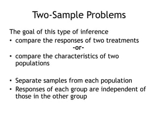
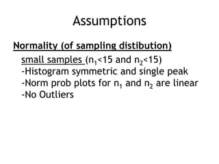
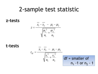
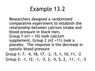
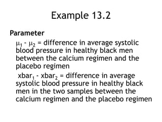
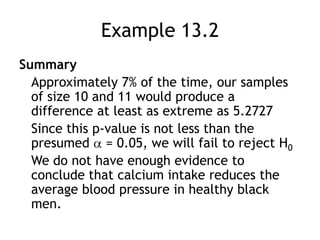
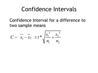
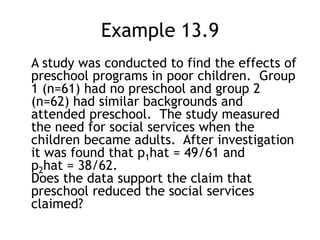
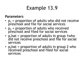
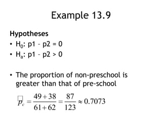
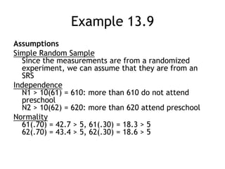
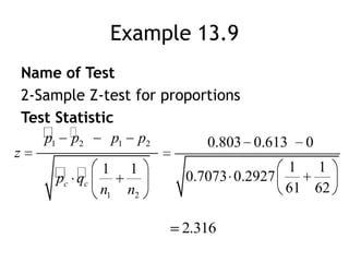
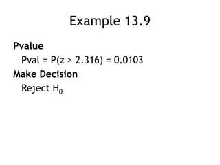
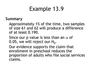
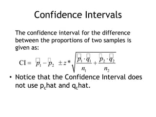
The document discusses comparing two population parameters using sample data. It covers comparing two means using a two-sample t-test or z-test, and comparing two proportions using a two-sample z-test. Key assumptions for these tests include independent random samples from each population and sample sizes large enough for the sampling distributions to be approximately normal. An example compares systolic blood pressure for two groups, one taking calcium and one placebo, and finds no significant difference. A second example finds preschool significantly reduces the proportion needing later social services.

1. Chapter 13Comparing Two Population Parameters

2. 13.1 Comparing Two Means

3. Two-Sample ProblemsThe goal of this type of inference compare the responses of two treatments -or-compare the characteristics of two populationsSeparate samples from each populationResponses of each group are independent of those in the other group

4. Before We BeginThis is another set of PHANTOMS proceduresIt is important to note that “two populations” means that there is no overlap in the samplesThe sample sizes do not need to be equal

5. HypothesesThere are two styles of writing hypothesesStyle 1H0: 1 = 2Ha: 1  2, orHa: 1 > 2, orHa: 1 < 2

6. HypothesesThere are two styles of writing hypothesesStyle 2H0: 1 - 2 = 0Ha: 1 - 2  0, orHa: 1 - 2 > 0 (this implies 1 > 2), orHa: 1 - 2 < 0 (this implies 1 < 2)

7. HypothesesThere are two styles of writing hypothesesStyle 2H0: 1 - 2 = 0Ha: 1 - 2  0, orHa: 1 - 2 > 0 (this implies 1 > 2), orHa: 1 - 2 < 0 (this implies 1 < 2)This style is more versatilesince it allows you to use adifference other than zero

8. AssumptionsSimple Random SampleEach sample must be from an SRSIndependenceSamples may not influence each otherNo paired data!N1 > 10n1and N2 > 10n2(if sampling w/o replacement)

9. AssumptionsNormality (of sampling distibution)large samples (n1 > 30 and n2 > 30)this is the Central Limit Theorem -OR-medium samples (15<n1<30 and 15<n2<30)-Histogram symmetric or slight skew and single peak-Norm prob plots for n1 and n2 are linear-No Outliers -OR-

10. AssumptionsNormality (of sampling distibution)small samples (n1<15 and n2<15)-Histogram symmetric and single peak-Norm prob plots for n1 and n2 are linear-No Outliers

11. 2-sample test statisticz-testst-testsdf = smaller of n1 -1 or n2 - 1

12. Example 13.2Researchers designed a randomized comparative experiment to establish the relationship between calcium intake and blood pressure in black men. Group 1 (n1 = 10) took calcium supplement, Group 2 (n2 =11) took a placebo. The response is the decrease in systolic blood pressureGroup 1: 7, -4, 18, 17, -3, -5, 1, 10, 11, -2Group 2: -1, 12, -1, -3, 3, -5, 5, 2, -11, -1, -3

13. Example 13.2Parameter 1 - 2 = difference in average systolic blood pressure in healthy black men between the calcium regimen and the placebo regimen xbar1 - xbar2 = difference in average systolic blood pressure in healthy black men in the two samples between the calcium regimen and the placebo regimen

14. Example 13.2HypothesesH0: 1 - 2 = 0Ha: 1 - 2 > 0

15. Example 13.2AssumptionsSimple Random SampleWe are told that both samples come from a randomized designIndependenceBoth samples are independent, and (n1) N1 > 10(10) =100, (n2) N2 > 10(11)=110the population of black men is greater than 110

16. Example 13.2Assumptions (cont)Sample 1Sample 2

17. Example 13.2Assumptions (cont)NormalityBoth samples are single peaked with moderate skewness and approximately normal with no outliers.Although sample 1 shows some skewness, the t-procedures are robust enough to handle this skew.

18. Example 13.2Name of TestWe will conduct a 2-sample t-test for population meansTest Statistic

19. Example 13.2P ValueDecisionFail to Reject H0 at the 5% significance level

20. Example 13.2SummaryApproximately 7% of the time, our samples of size 10 and 11 would produce a difference at least as extreme as 5.2727Since this p-value is not less than the presumed  = 0.05, we will fail to reject H0 We do not have enough evidence to conclude that calcium intake reduces the average blood pressure in healthy black men.

21. Confidence Intervals Confidence Interval for a difference to two sample means

22. Robustness 2-sample t-procedures are more robust than one sample procedures. They can be used for sample sizes as small as n1 = n2 = 5 when the samples have similar shapes.Guidelines for using t-proceduresn1 + n2< 15: data must be approx normal,no outliersn1 + n2 >15: data can have slight skew, no outliersn1 + n2> 30: data can have skew

23. Degrees of FreedomWe have been using the smaller of n1 or n2 to determine the dfThis will ensure that our pvalue is smaller than the calculated pvalueand confidence intervals are smaller than calculated.These are “worst case scenario” calculationsThere is a more exact df formula on p792Your calculator also uses a df formula for two samplesYou do not need to memorize these other formulas!

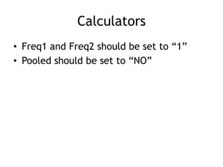
24. CalculatorsThe tests we are using are located in the [STAT] -> “TESTS” menu2-SampZTest = two sample z-test for means2-SampTTest = two sample t-test for mean2-SampZInt = two sample z Confidence Interval for difference of means2-SampTInt = two sample t Confidence Interval for difference of means

25. CalculatorsFreq1 and Freq2 should be set to “1”Pooled should be set to “NO”

26. 13.2 Comparing two Proportions

27. 2-Sample Inference for ProportionsWe are testing to see ifTwo populations have the same proportion ORA treatment affects the proportion Remember: this is not a procedure for paired data (matched pair design/pre- and post-test)

28. Combined ProportionOne of the underlying assumptions of the test is that the two proportions actually come from the same population.The test makes use of the “combined proportion” as below:

29. HypothesesThere are two styles of writing hypothesesStyle 1H0: p1 = p2Ha: p1  p2, orHa: p1 > p2, orHa: p1 < p2

30. HypothesesThere are two styles of writing hypothesesStyle 2H0: p1 - p2 = 0Ha: p1 - p2  0, orHa: p1 - p2 > 0 (this implies p1 > p2), orHa: p1 - p2 < 0 (this implies p1 < p2)

31. HypothesesThere are two styles of writing hypothesesStyle 2H0: p1 - p2 = 0Ha: p1 - p2  0, orHa: p1 - p2 > 0 (this implies p1 > p2), orHa: p1 - p2 < 0 (this implies p1 < p2)This style is more versatilesince it allows you to use adifference other than zero

32. AssumptionsSimple Random SampleBoth samples must be viewed as an SRS from their respective population or two groups from a randomized experimentIndependenceN1 > 10n1 and N2 > 10n2Normalityn1(pchat)> 5, n1(qchat)> 5 and n2(pchat)> 5, n2(qchat)> 5

33. Test StatisticThe test statistic for proportions is always from the Normal distribution 

34. Example 13.9 A study was conducted to find the effects of preschool programs in poor children. Group 1 (n=61) had no preschool and group 2 (n=62) had similar backgrounds and attended preschool. The study measured the need for social services when the children became adults. After investigation it was found that p1hat = 49/61 and p2hat = 38/62.Does the data support the claim that preschool reduced the social services claimed?

35. Example 13.9Parametersp1 = proportion of adults who did not receive preschool and file for social servicesp2 = proportion of adults who received preschool and filed for social servicesp1hat = proportion of adults in group 1who did not receive preschool and file for social servicesp2hat = proportion of adults in group 2 who received preschool and filed for social services

36. Example 13.9HypothesesH0: p1 – p2 = 0Ha: p1 – p2 > 0The proportion of non-preschool is greater than that of pre-school

37. Example 13.9AssumptionsSimple Random SampleSince the measurements are from a randomized experiment, we can assume that they are from an SRSIndependenceN1 > 10(61) = 610: more than 610 do not attend preschoolN2 > 10(62) = 620: more than 620 attend preschoolNormality61(.70) = 42.7 > 5, 61(.30) = 18.3 > 562(.70) = 43.4 > 5, 62(.30) = 18.6 > 5

38. Example 13.9Name of Test2-Sample Z-test for proportionsTest Statistic

39. Example 13.9PvaluePval = P(z > 2.316) = 0.0103Make DecisionReject H0

40. Example 13.9SummaryApproximately 1% of the time, two samples of size 61 and 62 will produce a difference of at least 0.190.Since our p value is less than an  of 0.05, we will reject our H0.Our evidence supports the claim that enrollment in preschool reduces the proportion of adults who file social services claims.

41. Confidence IntervalsThe confidence interval for the difference between the proportions of two samples is given as:Notice that the Confidence Interval does not use pchat and qchat.

42. Confidence IntervalsAssumptionsSimple Random SampleBoth samples must be viewed as an SRS from their respective population or two groups from a randomized experimentIndependenceN1 > 10n1 and N2 > 10n2Normality n1(p1)> 5, n1(q1)> 5 and n2(p2)> 5, n2(q2)> 5(again, not pc or qc)

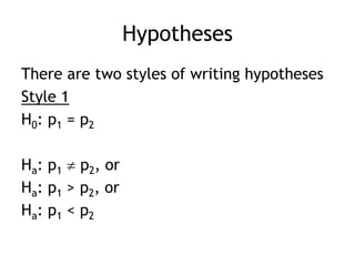
43. Calculators The tests we are using are located in the [STAT] -> “TESTS” menu2-PropZTest = 2 proportion z-test2-PropZInt = 2 proportion confidence interval