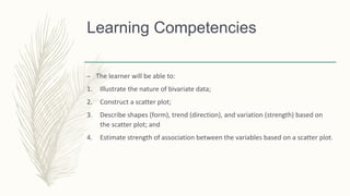
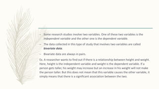
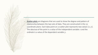
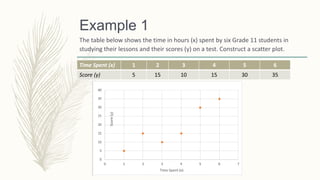
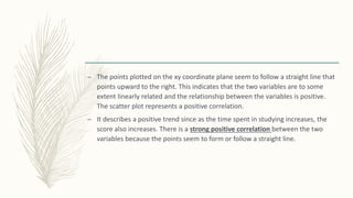
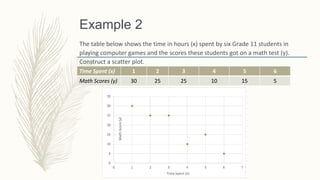
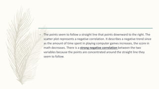
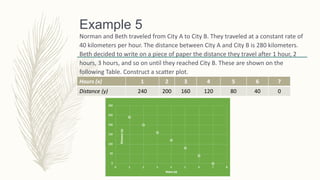
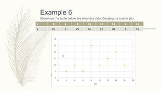
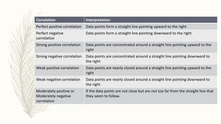
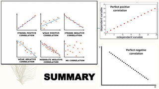
Scatter
Plots
Learning Competencies
– The learner will be able to:
1. Illustrate the nature of bivariate data;
2. Construct a scatter plot;
3. Describe shapes (form), trend (direction), and variation (strength) based on
the scatter plot; and
4. Estimate strength of association between the variables based on a scatter plot.
– Some research studies involve two variables. One of these two variables is the
independent variable and the other one is the dependent variable.
– The data collected in this type of study that involves two variables are called
bivariate data.
– Bivariate data are always in pairs.
Ex. A researcher wants to find out if there is a relationship between height and weight.
Here, height is the independent variable and weight is the dependent variable. If a
person gets taller, his weight may increase but an increase in his weight will not make
the person taller. But this does not mean that this variable causes the other variable, it
simply means that there is a significant association between the two.
– Scatter plots are diagrams that are used to show the degree and pattern of
relationship between the two sets of data. They are constructed in the 𝑥𝑦
coordinate plane. Each data point on a scatter plot represents two values 𝑥, 𝑦 .
The abscissa of the point is a value of the independent variable 𝑥 and the
ordinate is a value of the dependent variable 𝑦.
Example 1
The table below shows the time in hours (x) spent by six Grade 11 students in
studying their lessons and their scores (y) on a test. Construct a scatter plot.
Time Spent (x) 1 2 3 4 5 6
Score (y) 5 15 10 15 30 35
– The points plotted on the xy coordinate plane seem to follow a straight line that
points upward to the right. This indicates that the two variables are to some
extent linearly related and the relationship between the variables is positive.
The scatter plot represents a positive correlation.
– It describes a positive trend since as the time spent in studying increases, the
score also increases. There is a strong positive correlation between the two
variables because the points seem to form or follow a straight line.
Example 2
The table below shows the time in hours (x) spent by six Grade 11 students in
playing computer games and the scores these students got on a math test (y).
Construct a scatter plot.
Time Spent (x) 1 2 3 4 5 6
Math Scores (y) 30 25 25 10 15 5
– The points seem to follow a straight line that points downward to the right. The
scatter plot represents a negative correlation. It describes a negative trend since
as the amount of time spent in playing computer games increases, the score in
math decreases. There is a strong negative correlation between the two
variables because the points are concentrated around the straight line they
seem to follow.
Example 3
The table below shows the number of selfies (x) posted online of students and the
scores (y) they obtained from a Science test. Construct a scatter plot.
Number of Selfies (x) 1 2 3 4 5 6
Scores in Science Test (y) 25 5 20 40 25 9
– Looking at the scatter plot, it can be noticed that the plotted data points are
neither following a straight line pointing upward or downward to the right nor
have a pattern. There is no correlation between numbers of selfies posted
online and the scores obtained in a Science test.
Example 4
The table below shows the number of composition notebooks and the
corresponding costs. The cost per composition notebook is Php 25. Construct a
scatter plot using these data.
Number of Notebooks (x) 1 2 3 4 5 6
Cost (y) 25 50 75 100 125 150
– The points are all on a straight line that points upward to the right. There is a
perfect positive correlation between the two variables. This is so because the
two variables are linear combinations of each other, 𝑦 = 25𝑥.
Example 5
Norman and Beth traveled from City A to City B. They traveled at a constant rate of
40 kilometers per hour. The distance between City A and City B is 280 kilometers.
Beth decided to write on a piece of paper the distance they travel after 1 hour, 2
hours, 3 hours, and so on until they reached City B. These are shown on the
following Table. Construct a scatter plot.
Hours (x) 1 2 3 4 5 6 7
Distance (y) 240 200 160 120 80 40 0
– All the points in the scatter plot are on a straight line that points downward to
the right. There is a perfect negative correlation between the two variables. As
the time traveled increases, the distance that needs to be traveled decreases.
Also, the relationship of the two variables can be expresses in linear equation,
𝑦 = 280 − 40𝑥.
Example 6
Shown on the table below are bivariate data. Construct a scatter plot.
x 4 2 8 10 12 14 6 16
y 10 5 25 10 15 20 5 10
– The points in the scatter plot seem to follow a straight line that points upward
to the right at certain intervals. However, it cannot be said that the correlation
is perfect positive not even moderately positive. There is a weak positive
correlation between the two variables because the data points are widely
spread and far from the straight line they seem to follow.
Correlation Interpretation
Perfect positive correlation Data points form a straight line pointing upward to the right
Perfect negative
correlation
Data points form a straight line pointing downward to the right
Strong positive correlation Data points are concentrated around a straight line pointing upward to the
right
Strong negative correlation Data points are concentrated around a straight line pointing downward to
the right
Weak positive correlation Data points are nearly closed around a straight line pointing upward to the
right
Weak negative correlation Data points are nearly closed around a straight line pointing downward to
the right
Moderately positive or
Moderately negative
correlation
If the data points are not close but are not too far from the straight line that
they seem to follow.
Perfect positive
correlation
Perfect negative
correlation
SUMMARY

SCATTER PLOTS

  • 1.
  • 2.
    Learning Competencies – Thelearner will be able to: 1. Illustrate the nature of bivariate data; 2. Construct a scatter plot; 3. Describe shapes (form), trend (direction), and variation (strength) based on the scatter plot; and 4. Estimate strength of association between the variables based on a scatter plot.
  • 3.
    – Some researchstudies involve two variables. One of these two variables is the independent variable and the other one is the dependent variable. – The data collected in this type of study that involves two variables are called bivariate data. – Bivariate data are always in pairs. Ex. A researcher wants to find out if there is a relationship between height and weight. Here, height is the independent variable and weight is the dependent variable. If a person gets taller, his weight may increase but an increase in his weight will not make the person taller. But this does not mean that this variable causes the other variable, it simply means that there is a significant association between the two.
  • 4.
    – Scatter plotsare diagrams that are used to show the degree and pattern of relationship between the two sets of data. They are constructed in the 𝑥𝑦 coordinate plane. Each data point on a scatter plot represents two values 𝑥, 𝑦 . The abscissa of the point is a value of the independent variable 𝑥 and the ordinate is a value of the dependent variable 𝑦.
  • 5.
    Example 1 The tablebelow shows the time in hours (x) spent by six Grade 11 students in studying their lessons and their scores (y) on a test. Construct a scatter plot. Time Spent (x) 1 2 3 4 5 6 Score (y) 5 15 10 15 30 35
  • 6.
    – The pointsplotted on the xy coordinate plane seem to follow a straight line that points upward to the right. This indicates that the two variables are to some extent linearly related and the relationship between the variables is positive. The scatter plot represents a positive correlation. – It describes a positive trend since as the time spent in studying increases, the score also increases. There is a strong positive correlation between the two variables because the points seem to form or follow a straight line.
  • 7.
    Example 2 The tablebelow shows the time in hours (x) spent by six Grade 11 students in playing computer games and the scores these students got on a math test (y). Construct a scatter plot. Time Spent (x) 1 2 3 4 5 6 Math Scores (y) 30 25 25 10 15 5
  • 8.
    – The pointsseem to follow a straight line that points downward to the right. The scatter plot represents a negative correlation. It describes a negative trend since as the amount of time spent in playing computer games increases, the score in math decreases. There is a strong negative correlation between the two variables because the points are concentrated around the straight line they seem to follow.
  • 9.
    Example 3 The tablebelow shows the number of selfies (x) posted online of students and the scores (y) they obtained from a Science test. Construct a scatter plot. Number of Selfies (x) 1 2 3 4 5 6 Scores in Science Test (y) 25 5 20 40 25 9
  • 10.
    – Looking atthe scatter plot, it can be noticed that the plotted data points are neither following a straight line pointing upward or downward to the right nor have a pattern. There is no correlation between numbers of selfies posted online and the scores obtained in a Science test.
  • 11.
    Example 4 The tablebelow shows the number of composition notebooks and the corresponding costs. The cost per composition notebook is Php 25. Construct a scatter plot using these data. Number of Notebooks (x) 1 2 3 4 5 6 Cost (y) 25 50 75 100 125 150
  • 12.
    – The pointsare all on a straight line that points upward to the right. There is a perfect positive correlation between the two variables. This is so because the two variables are linear combinations of each other, 𝑦 = 25𝑥.
  • 13.
    Example 5 Norman andBeth traveled from City A to City B. They traveled at a constant rate of 40 kilometers per hour. The distance between City A and City B is 280 kilometers. Beth decided to write on a piece of paper the distance they travel after 1 hour, 2 hours, 3 hours, and so on until they reached City B. These are shown on the following Table. Construct a scatter plot. Hours (x) 1 2 3 4 5 6 7 Distance (y) 240 200 160 120 80 40 0
  • 14.
    – All thepoints in the scatter plot are on a straight line that points downward to the right. There is a perfect negative correlation between the two variables. As the time traveled increases, the distance that needs to be traveled decreases. Also, the relationship of the two variables can be expresses in linear equation, 𝑦 = 280 − 40𝑥.
  • 15.
    Example 6 Shown onthe table below are bivariate data. Construct a scatter plot. x 4 2 8 10 12 14 6 16 y 10 5 25 10 15 20 5 10
  • 16.
    – The pointsin the scatter plot seem to follow a straight line that points upward to the right at certain intervals. However, it cannot be said that the correlation is perfect positive not even moderately positive. There is a weak positive correlation between the two variables because the data points are widely spread and far from the straight line they seem to follow.
  • 17.
    Correlation Interpretation Perfect positivecorrelation Data points form a straight line pointing upward to the right Perfect negative correlation Data points form a straight line pointing downward to the right Strong positive correlation Data points are concentrated around a straight line pointing upward to the right Strong negative correlation Data points are concentrated around a straight line pointing downward to the right Weak positive correlation Data points are nearly closed around a straight line pointing upward to the right Weak negative correlation Data points are nearly closed around a straight line pointing downward to the right Moderately positive or Moderately negative correlation If the data points are not close but are not too far from the straight line that they seem to follow.
  • 18.

Editor's Notes

  • #4 The heights of the students which may be in centimeters and the weights of the students which may be in kilograms are the bivariate data.