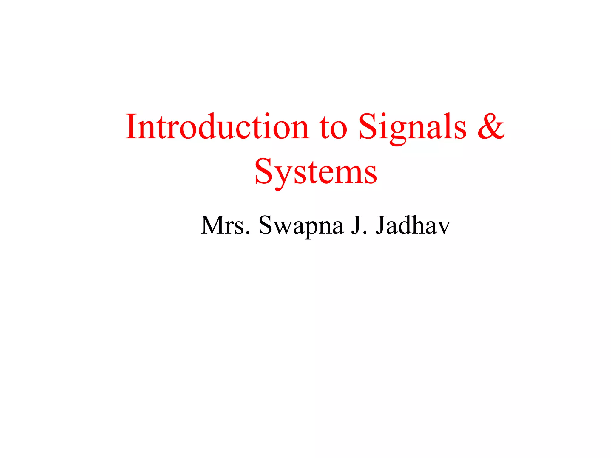
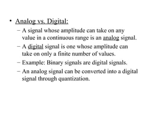
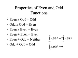
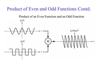
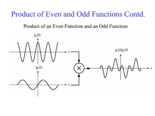
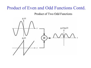
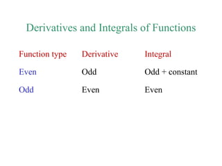
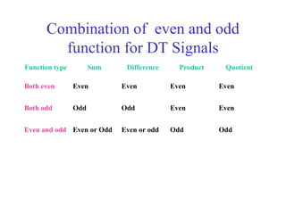
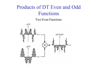
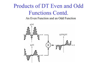
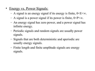
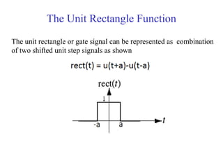
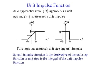
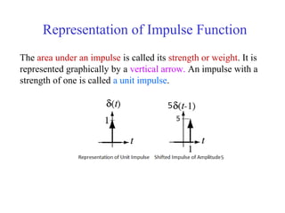
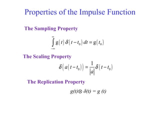
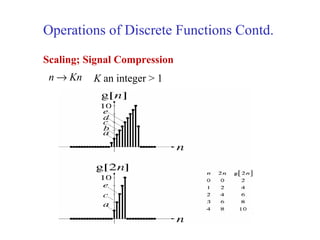
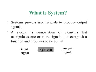
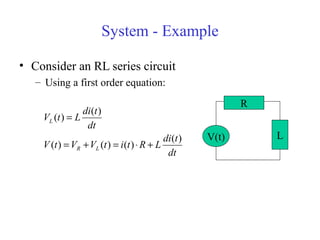
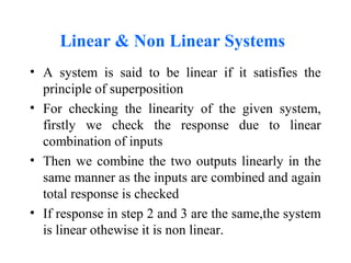
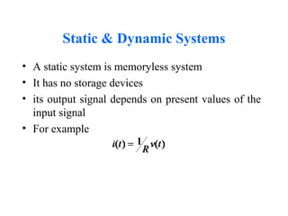
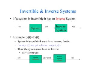
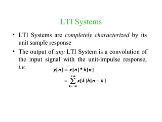
This document provides an introduction to signals and systems. It defines a signal as a function that carries information about a physical phenomenon, and a system as an entity that processes signals to produce new outputs. Signals can be classified as continuous or discrete, deterministic or random, periodic or aperiodic, even or odd, energy-based or power-based, and causal or noncausal. The document discusses examples and properties of different signal types and how systems manipulate inputs to generate outputs. It covers key concepts like energy, power, periodicity, causality, and system modeling that are important foundations for signals and systems analysis.

1. Introduction to Signals &
Systems
Mrs. Swapna J. Jadhav

2. Introduction to Signals
• A Signal is the function of one or more independent
variables that carries some information to represent a
physical phenomenon.
• A continuous-time signal, also called an analog signal, is
defined along a continuum of time.

3. Signals
• Signals are functions of independent variables; time (t) or
space (x,y)
• A physical signal is modeled using mathematical
functions.
• Examples:
– Electrical signals: Voltages/currents in a circuit v(t),i(t)
– Temperature (may vary with time/space)
– Acoustic signals: audio/speech signals (varies with time)
– Video (varies with time and space)
– Biological signals: Heartbeat, EEG

4. Systems
• A system is an entity that manipulates one or more signals
that accomplish a function, thereby yielding new signals.
• The input/output relationship of a system is modeled using
mathematical equations.
• We want to study the response of systems to signals.
• A system may be made up of physical components
(electrical, mechanical, hydraulic) or may be an algorithm
that computes an output from an input signal.
• Examples:
– Circuits (Input: Voltage, Output: Current)
• Simple resistor circuit:
– Mass Spring System (Input: Force, Output: displacement)
– Automatic Speaker Recognition (Input: Speech, Output: Identity)
)()( tRitv =

5. Applications of Signals and Systems
• Acoustics: Restore speech in a noisy environment such as
cockpit
• Communications: Transmission in mobile phones, GPS,
radar and sonar
• Multimedia: Compress signals to store data such as CDs,
DVDs
• Biomedical: Extract information from biological signals:
– Electrocardiogram (ECG) electrical signals generated by the heart
– Electroencephalogram (EEG) electrical signals generated by the
brain
– Medical Imaging
• Biometrics: Fingerprint identification, speaker recognition,
iris recognition

6. Classification of Signals
Major classifications of the signal
• Continuous time signal
• Discrete time signal

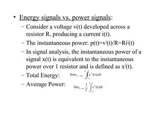
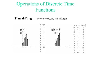
7. • Continuous-time vs. discrete-time:
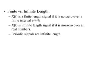
– A signal is continuous time if it is defined for
all time, x(t).
– A signal is discrete time if it is defined only at
discrete instants of time, x[n].
– A discrete time signal is derived from a
continuous time signal through sampling, i.e.:
periodsamplingisTnTxnx ss ),(][ =

8. Classification of Signals
• One-dimensional vs. Multi-dimensional:
The signal can be a function of a single
variable or multiple variables.
– Examples:
• Speech varies as a function of timeone-
dimensional
• Image intensity varies as a function of (x,y)
coordinatesmulti-dimensional
– In this course, we focus on one-dimensional
signals.

9. • Analog vs. Digital:
– A signal whose amplitude can take on any
value in a continuous range is an analog signal.
– A digital signal is one whose amplitude can
take on only a finite number of values.
– Example: Binary signals are digital signals.
– An analog signal can be converted into a digital
signal through quantization.

10. • Deterministic vs. Random:
– A signal is deterministic if we can define its
value at each time point as a mathematical
function
– A signal is random if it cannot be described by
a mathematical function (can only define
statistics)
– Example:
• Electrical noise generated in an amplifier of a
radio/TV receiver.

11. Deterministic & Non Deterministic Signals
Deterministic signals
• Behavior of these signals is predictable w.r.t time
• There is no uncertainty with respect to its value at any
time.
• These signals can be expressed mathematically.
For example x(t) = sin(3t) is deterministic signal.

12. Deterministic & Non Deterministic Signals
Contd.
Non Deterministic or Random signals
• Behavior of these signals is random i.e. not predictable
w.r.t time.
• There is an uncertainty with respect to its value at any
time.
• These signals can’t be expressed mathematically.
• For example Thermal Noise generated is non
deterministic signal.

13. Classification of Signals
classifications of the signal in Continuous
time and Discrete time signal
• Periodic and Aperiodic signal
• Even and Odd signal
• Energy and Power signal
• Causal and non-Causal
• Sinusoidal and Exponential

14. • Periodic vs. Aperiodic Signals:
– A periodic signal x(t) is a function of time that satisfies
– The smallest T, that satisfies this relationship is called
the fundamental period.
– is called the frequency of the signal (Hz).
– Angular frequency, (radians/sec).
– A signal is either periodic or aperiodic.
– A periodic signal must continue forever.
– Example: The voltage at an AC power source is
periodic.
)()( Ttxtx +=
T
f
1
=
∫ ∫ ∫
+ +
==
0 0
0
)()()(
Ta
a
Tb
b T
dttxdttxdttx
T
f
π
πω
2
2 ==

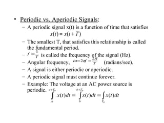
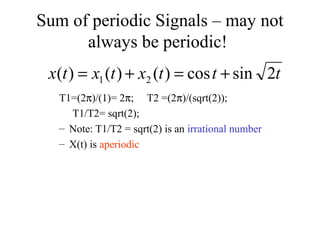
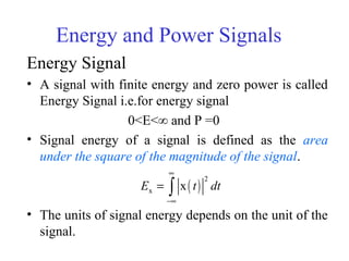
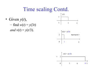
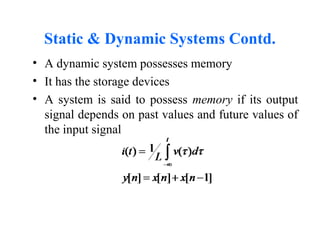
15. Periodic and Non-periodic Signals
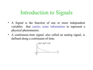
• Given x(t) is a continuous-time signal
• x (t) is periodic if x(t) = x(t+Tₒ) for any T and any integer n
• Example
– x(t) = A cos(ωt)
– x(t+Tₒ) = A cos[ω(t+Tₒ)] = A cos(ωt+ωTₒ)= A cos(ωt+2π)
= A cos(ωt)
– Note: Tₒ =1/fₒ ; ω=2πfₒ

16. Periodic and Non-periodic Signals
Contd.
• For non-periodic signals
x(t) ≠ x(t+Tₒ)
• A non-periodic signal is assumed to have a
period T = ∞
• Example of non periodic signal is an
exponential signal

17. Important Condition of Periodicity for
Discrete Time Signals
• A discrete time signal is periodic if
x(n) = x(n+N)
• For satisfying the above condition the
frequency of the discrete time signal should
be ratio of two integers
i.e. fₒ = k/N

18. Sum of periodic Signals – may not
always be periodic!
T1=(2π)/(1)= 2π; T2 =(2π)/(sqrt(2));
T1/T2= sqrt(2);
– Note: T1/T2 = sqrt(2) is an irrational number
– X(t) is aperiodic
tttxtxtx 2sincos)()()( 21 +=+=

19. Periodic Signals

20. Aperiodic Signals

21. • Even vs. Odd:
– A signal is even if x(t)=x(-t).
– A signal is odd if x(t)=-x(-t)
– Examples:
• Sin(t) is an odd signal.
• Cos(t) is an even signal.
– A signal can be even, odd or neither.
– Any signal can be written as a combination of an
even and odd signal.
2
)()(
)(
2
)()(
)(
txtx
tx
txtx
tx
o
e
−−
=
−+
=

22. Properties of Even and Odd
Functions
• Even x Odd = Odd
• Odd x Odd = Even
• Even x Even = Even
• Even + Even = Even
• Even + Odd = Neither
• Odd + Odd = Odd
0)(
)(2)(
0
=
=
∫
∫∫
−
−
dttx
dttxdttx
a
a
o
a
e
a
a
e

23. Even and Odd Parts of Functions
( )
( ) ( )g g
The of a function is g
2
e
t t
t
+ −
=even part
( )
( ) ( )g g
The of a function is g
2
o
t t
t
− −
=odd part
A function whose even part is zero, is odd and a function
whose odd part is zero, is even.

24. Various Combinations of even and odd
functions
Function type Sum Difference Product Quotient
Both even Even Even Even Even
Both odd Odd Odd Even Even
Even and odd Neither Neither Odd Odd

25. Product of Two Even Functions
Product of Even and Odd Functions

26. Product of Even and Odd Functions Contd.
Product of an Even Function and an Odd Function

27. Product of an Even Function and an Odd Function
Product of Even and Odd Functions Contd.

28. Product of Two Odd Functions
Product of Even and Odd Functions Contd.

29. Derivatives and Integrals of Functions
Function type Derivative Integral
Even Odd Odd + constant
Odd Even Even

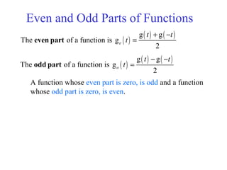
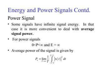
30. Discrete Time Even and Odd Signals
[ ]
[ ] [ ]g g
g
2
e
n n
n
+ −
= [ ]
[ ] [ ]g g
g
2
o
n n
n
− −
=
[ ] [ ]g gn n= − [ ] [ ]g gn n= − −

31. Combination of even and odd
function for DT Signals
Function type Sum Difference Product Quotient
Both even Even Even Even Even
Both odd Odd Odd Even Even
Even and odd Even or Odd Even or odd Odd Odd

32. Products of DT Even and Odd
Functions
Two Even Functions

33. Products of DT Even and Odd
Functions Contd.
An Even Function and an Odd Function

34. • Finite vs. Infinite Length:
– X(t) is a finite length signal if it is nonzero over a
finite interval a<t<b
– X(t) is infinite length signal if it is nonzero over all
real numbers.
– Periodic signals are infinite length.

35. • Energy signals vs. power signals:
– Consider a voltage v(t) developed across a
resistor R, producing a current i(t).
– The instantaneous power: p(t)=v2
(t)/R=Ri2
(t)
– In signal analysis, the instantaneous power of a
signal x(t) is equivalent to the instantaneous
power over 1 resistor and is defined as x2
(t).
– Total Energy:
– Average Power:
∫−
∞→
2/
2/
2
)(
1
lim
T
T
T dttx
T
∫−
∞→
2/
2/
2
)(lim
T
T
T dttx

36. Energy and Power Signals
Energy Signal
• A signal with finite energy and zero power is called
Energy Signal i.e.for energy signal
0<E<∞ and P =0
• Signal energy of a signal is defined as the area
under the square of the magnitude of the signal.
• The units of signal energy depends on the unit of the
signal.
( )
2
x xE t dt
∞
−∞
= ∫

37. Energy and Power Signals Contd.
Power Signal
• Some signals have infinite signal energy. In that
case it is more convenient to deal with average
signal power.
• For power signals
0<P<∞ and E = ∞
• Average power of the signal is given by
( )
/ 2
2
x
/ 2
1
lim x
T
T
T
P t dt
T→∞
−
= ∫

38. Energy and Power Signals Contd.
• For a periodic signal x(t) the average signal
power is
• T is any period of the signal.
• Periodic signals are generally power signals.
( )
2
x
1
x
T
P t dt
T
= ∫

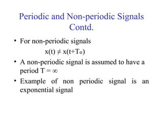
39. Signal Energy and Power for DT
Signal
•The signal energy of a for a discrete time signal x[n] is
[ ]
2
x x
n
E n
∞
=−∞
= ∑
•A discrete time signal with finite energy and zero
power is called Energy Signal i.e.for energy signal
0<E<∞ and P =0

40. Signal Energy and Power for DT
Signal Contd.
The average signal power of a discrete time power signal
x[n] is
[ ]
1
2
x
1
lim x
2
N
N
n N
P n
N
−
→∞
=−
= ∑
[ ]
2
x
1
x
n N
P n
N =
= ∑
For a periodic signal x[n] the average signal power is
The notation means the sum over any set of
consecutive 's exactly in length.
n N
n N
=
 
 ÷
 ÷
 
∑

41. • Energy vs. Power Signals:
– A signal is an energy signal if its energy is finite, 0<E<∞.
– A signal is a power signal if its power is finite, 0<P<∞.
– An energy signal has zero power, and a power signal has
infinite energy.
– Periodic signals and random signals are usually power
signals.
– Signals that are both deterministic and aperiodic are
usually energy signals.
– Finite length and finite amplitude signals are energy
signals.

42. • Causal, Anticausal vs. Noncausal Signals:
– A signal that does not start before t=0 is a
causal signal. x(t)=0, t<0
– A signal that starts before t=0 is a noncausal
signal.
– A signal that is zero for t>0 is called an
anticausal signal.

43. Elementary Signals
Sinusoidal & Exponential Signals
• Sinusoids and exponentials are important in signal and
system analysis because they arise naturally in the
solutions of the differential equations.
• Sinusoidal Signals can expressed in either of two ways :
cyclic frequency form- A sin 2Пfot = A sin(2П/To)t
radian frequency form- A sin ωot
ωo= 2Пfo= 2П/To
To= Time Period of the Sinusoidal Wave

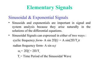
44. Sinusoidal & Exponential Signals Contd.
x(t) = A sin (2Пfot+ θ)
= A sin (ωot+ θ)
x(t) = Aeat Real Exponential
= Aejω̥t =
A[cos (ωot) +j sin (ωot)] ComplexExponential
θ = Phase of sinusoidal wave
A = amplitude of a sinusoidal or exponential signal
fo= fundamental cyclic frequency of sinusoidal signal
ωo= radian frequency
Sinusoidal signal

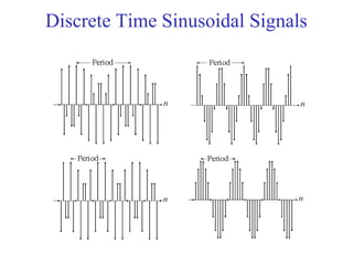
45. Discrete Time Exponential and
Sinusoidal Signals
• DT signals can be defined in a manner analogous to their
continuous-time counter part
x[n] = A sin (2Пn/No+θ)
= A sin (2ПFon+ θ)
x[n] = an
n = the discrete time
A = amplitude
θ = phase shifting radians,
No = Discrete Period of the wave
1/N0= Fo= Ωo/2 П = Discrete Frequency
Discrete Time Sinusoidal Signal
Discrete Time Exponential Signal

46. Discrete Time Sinusoidal Signals

47. Unit Step Function
( )
1 , 0
u 1/ 2 , 0
0 , 0
t
t t
t
>

= =
 <
Precise Graph Commonly-Used Graph

48. Discrete Time Unit Step Function or
Unit Sequence Function
[ ]
1 , 0
u
0 , 0
n
n
n
≥
= 
<

49. Signum Function
( ) ( )
1 , 0
sgn 0 , 0 2u 1
1 , 0
t
t t t
t
> 
 
= = = − 
 − < 
Precise Graph Commonly-Used Graph
The signum function, is closely related to the unit-step
function.

50. Unit Ramp Function
( ) ( ) ( )
, 0
ramp u u
0 , 0
t
t t
t d t t
t
λ λ
−∞
> 
= = = 
≤ 
∫
•The unit ramp function is the integral of the unit step function.
•It is called the unit ramp function because for positive t, its
slope is one amplitude unit per time.

51. Discrete Time Unit Ramp Function
[ ] [ ]
, 0
ramp u 1
0 , 0
n
m
n n
n m
n =−∞
≥ 
= = − 
< 
∑

52. Rectangular Pulse or Gate Function
Rectangular pulse, ( )
1/ , / 2
0 , / 2
a
a t a
t
t a
δ
 <
= 
>

53. The Unit Rectangle Function
The unit rectangle or gate signal can be represented as combination
of two shifted unit step signals as shown

54. Unit Impulse Function
( )
( )
As approaches zero, g approaches a unit
step andg approaches a unit impulse
a t
t′
So unit impulse function is the derivative of the unit step
function or unit step is the integral of the unit impulse
function
Functions that approach unit step and unit impulse

55. Representation of Impulse Function
The area under an impulse is called its strength or weight. It is
represented graphically by a vertical arrow. An impulse with a
strength of one is called a unit impulse.

56. Properties of the Impulse Function
( ) ( ) ( )0 0g gt t t dt tδ
∞
−∞
− =∫
The Sampling Property
( )( ) ( )0 0
1
a t t t t
a
δ δ− = −
The Scaling Property
The Replication Property
g(t)⊗ δ(t) = g (t)

57. Unit Impulse Train
The unit impulse train is a sum of infinitely uniformly-
spaced impulses and is given by
( ) ( ) , an integerT
n
t t nT nδ δ
∞
=−∞
= −∑

58. Discrete Time Unit Impulse Function or
Unit Pulse Sequence
[ ]
1 , 0
0 , 0
n
n
n
δ
=
= 
≠
[ ] [ ] for any non-zero, finite integer .n an aδ δ=

59. Unit Pulse Sequence Contd.
• The discrete-time unit impulse is a function in the
ordinary sense in contrast with the continuous-
time unit impulse.
• It has a sampling property.
• It has no scaling property i.e.
δ[n]= δ[an] for any non-zero finite integer ‘a’

60. Sinc Function
( )
( )sin
sinc
t
t
t
π
π
=

61. The Unit Triangle Function
A triangular pulse whose height and area are both one but its base
width is not, is called unit triangle function. The unit triangle is
related to the unit rectangle through an operation called
convolution.

62. Operations of Signals
• Sometime a given mathematical function may
completely describe a signal .
• Different operations are required for different
purposes of arbitrary signals.
• The operations on signals can be
Time Shifting
Time Scaling
Time Inversion or Time Folding

63. Time Shifting
• The original signal x(t) is shifted by an
amount tₒ.
• X(t)X(t-to) Signal Delayed Shift to the
right

64. Time Shifting Contd.
• X(t)X(t+to) Signal Advanced Shift
to the left

65. Time Scaling
• For the given function x(t), x(at) is the time
scaled version of x(t)
• For a 1,period of function x(t) reduces and˃
function speeds up. Graph of the function
shrinks.
• For a 1, the period of the x(t) increases˂
and the function slows down. Graph of the
function expands.

66. Time scaling Contd.
Example: Given x(t) and we are to find y(t) = x(2t).
The period of x(t) is 2 and the period of y(t) is 1,

67. Time scaling Contd.
• Given y(t),
– find w(t) = y(3t)
and v(t) = y(t/3).

68. Time Reversal
• Time reversal is also called time folding
• In Time reversal signal is reversed with
respect to time i.e.
y(t) = x(-t) is obtained for the given
function

69. Time reversal Contd.

70. 0 0, an integern n n n→ +Time shifting
Operations of Discrete Time
Functions

71. Operations of Discrete Functions Contd.
Scaling; Signal Compression
n Kn→ K an integer > 1

72. What is System?
• Systems process input signals to produce output
signals
• A system is combination of elements that
manipulates one or more signals to accomplish a
function and produces some output.
system output
signal
input
signal

73. Examples of Systems
– A circuit involving a capacitor can be viewed as a
system that transforms the source voltage (signal) to the
voltage (signal) across the capacitor
– A communication system is generally composed of three
sub-systems, the transmitter, the channel and the
receiver. The channel typically attenuates and adds
noise to the transmitted signal which must be processed
by the receiver
– Biomedical system resulting in biomedical signal
processing
– Control systems

74. System - Example
• Consider an RL series circuit
– Using a first order equation:
dt
tdi
LRtitVVtV
dt
tdi
LtV
LR
L
)(
)()()(
)(
)(
+⋅=+=
=
LV(t)
R

75. Mathematical Modeling of Continuous
Systems
Most continuous time systems represent how continuous
signals are transformed via differential equations.
E.g. RC circuit
System indicating car velocity
)(
1
)(
1)(
tv
RC
tv
RCdt
tdv
sc
c
=+
)()(
)(
tftv
dt
tdv
m =+ ρ

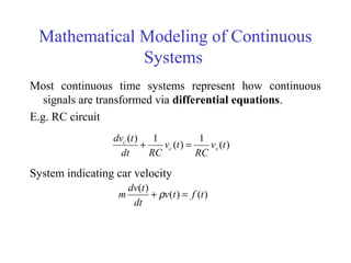
76. Mathematical Modeling of Discrete
Time Systems
Most discrete time systems represent how discrete signals are
transformed via difference equations
e.g. bank account, discrete car velocity system
][]1[01.1][ nxnyny +−=
][]1[][ nf
m
nv
m
m
nv
∆+
∆
=−
∆+
−
ρρ

77. Order of System
• Order of the Continuous System is the highest
power of the derivative associated with the output
in the differential equation
• For example the order of the system shown is 1.
)()(
)(
tftv
dt
tdv
m =+ ρ

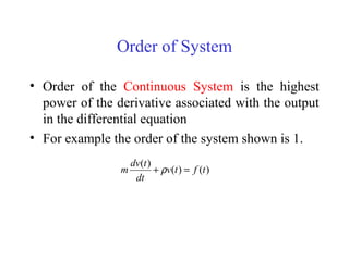
78. Order of System Contd.
• Order of the Discrete Time system is the
highest number in the difference equation
by which the output is delayed
• For example the order of the system shown
is 1.
][]1[01.1][ nxnyny +−=

79. Interconnected Systems
notes
• Parallel
• Serial (cascaded)
• Feedback
LV(t)
R
L
C

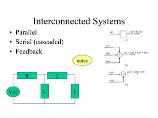
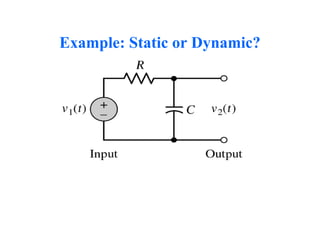
80. Interconnected System Example
• Consider the following systems with 4 subsystem
• Each subsystem transforms it input signal
• The result will be:
– y3(t)=y1(t)+y2(t)=T1[x(t)]+T2[x(t)]
– y4(t)=T3[y3(t)]= T3(T1[x(t)]+T2[x(t)])
– y(t)= y4(t)* y5(t)= T3(T1[x(t)]+T2[x(t)])* T4[x(t)]

81. Feedback System
• Used in automatic control
– e(t)=x(t)-y3(t)= x(t)-T3[y(t)]=
– y(t)= T2[m(t)]=T2(T1[e(t)])
  y(t)=T2(T1[x(t)-y3(t)])= T2(T1( [x(t)] - T3[y(t)] ) ) =
– =T2(T1([x(t)] –T3[y(t)]))

82. Types of Systems
• Causal & Anticausal
• Linear & Non Linear
• Time Variant &Time-invariant
• Stable & Unstable
• Static & Dynamic
• Invertible & Inverse Systems

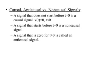
83. Causal & Anticausal Systems
• Causal system : A system is said to be causal if
the present value of the output signal depends only
on the present and/or past values of the input
signal.
• Example: y[n]=x[n]+1/2x[n-1]

84. Causal & Anticausal Systems Contd.
• Anticausal system : A system is said to be
anticausal if the present value of the output
signal depends only on the future values of
the input signal.
• Example: y[n]=x[n+1]+1/2x[n-1]

85. Linear & Non Linear Systems
• A system is said to be linear if it satisfies the
principle of superposition
• For checking the linearity of the given system,
firstly we check the response due to linear
combination of inputs
• Then we combine the two outputs linearly in the
same manner as the inputs are combined and again
total response is checked
• If response in step 2 and 3 are the same,the system
is linear othewise it is non linear.

86. Time Invariant and Time Variant
Systems
• A system is said to be time invariant if a time
delay or time advance of the input signal leads to a
identical time shift in the output signal.

87. Stable & Unstable Systems
• A system is said to be bounded-input bounded-
output stable (BIBO stable) if every bounded
input results in a bounded output.

88. Stable & Unstable Systems Contd.
Example
- y[n]=1/3(x[n]+x[n-1]+x[n-2])
1
[ ] [ ] [ 1] [ 2]
3
1
(| [ ]| | [ 1]| | [ 2]|)
3
1
( )
3
x x x x
y n x n x n x n
x n x n x n
M M M M
= + − + −
≤ + − + −
≤ + + =

89. Stable & Unstable Systems Contd.
Example: The system represented by
y(t) = A x(t) is unstable ; A 1˃
Reason: let us assume x(t) = u(t), then at
every instant u(t) will keep on multiplying
with A and hence it will not be bonded.

90. Static & Dynamic Systems
• A static system is memoryless system
• It has no storage devices
• its output signal depends on present values of the
input signal
• For example

91. Static & Dynamic Systems Contd.
• A dynamic system possesses memory
• It has the storage devices
• A system is said to possess memory if its output
signal depends on past values and future values of
the input signal

92. Example: Static or Dynamic?

93. Example: Static or Dynamic?
Answer:
• The system shown above is RC circuit
• R is memoryless
• C is memory device as it stores charge
because of which voltage across it can’t
change immediately
• Hence given system is dynamic or memory
system

94. Invertible & Inverse Systems
• If a system is invertible it has an Inverse System
• Example: y(t)=2x(t)
– System is invertible must have inverse, that is:
– For any x(t) we get a distinct output y(t)
– Thus, the system must have an Inverse
• x(t)=1/2 y(t)=z(t)
y(t)
System
Inverse
System
x(t) x(t)
y(t)=2x(t)System
(multiplier)
Inverse
System
(divider)
x(t) x(t)

95. LTI Systems
• LTI Systems are completely characterized by its
unit sample response
• The output of any LTI System is a convolution of
the input signal with the unit-impulse response,
i.e.

96. Properties of Convolution
Commutative Property
][*][][*][ nxnhnhnx =
Distributive Property
])[*][(])[*][(
])[][(*][
21
21
nhnxnhnx
nhnhnx
+
=+
Associative Property
][*])[*][(
][*])[*][(
][*][*][
12
21
21
nhnhnx
nhnhnx
nhnhnx
=
=

97. Useful Properties of (DT) LTI Systems
• Causality:
• Stability:
Bounded Input ↔ Bounded Output
00][ <= nnh
∞<∑
∞
−∞=k
kh ][
∞<−≤−=
∞<≤
∑∑
∞
−∞=
∞
−∞= kk
knhxknhkxny
xnx
][][][][
][for
max
max