Classification of-signals-systems-ppt

Classification of Signals &
Systems

Introduction to Signals
• A Signal is the function of one or more independent
variables that carries some information to represent a
physical phenomenon.
e.g. ECG, EEG
• Two Types of Signals
1. Continuous-time signals
2. Discrete-time signals

3
1. Continuous-Time Signals
• Signal that has a value for all points in time
• Function of time
– Written as x(t) because the signal “x” is a function of time
• Commonly found in the physical world
– ex. Human speech
• Displayed graphically as a line
x(t)
t

4
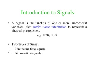
2. Discrete-Time Signals
• Signal that has a value for only specific points in time
• Typically formed by “sampling” a continuous-time signal
– Taking the value of the original waveform at specific intervals in time
• Function of the sample value, n
– Write as x[n]
– Often called a sequence
• Commonly found in the digital world
– ex. wav file or mp3
• Displayed graphically as individual values
– Called a “stem” plot
x[n]
n1 2 3 4 5 6 7 8 9 10
Sample number

5
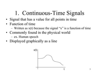
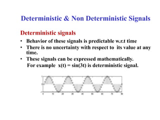
Examples: CT vs. DT Signals
( )x t [ ]x n
nt

6
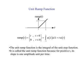
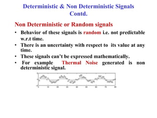
• Discrete-time signals are often obtained by
sampling continuous-time signals
Sampling
( )x t [ ] ( ) ( )t nTx n x t x nT . .

Unit Ramp Function
     
, 0
ramp u u
0 , 0
t
t t
t d t t
t
 

 
   
 

•The unit ramp function is the integral of the unit step function.
•It is called the unit ramp function because for positive t, its
slope is one amplitude unit per time.

Unit Impulse Function
 
 
As approaches zero, g approaches a unit
step andg approaches a unit impulse
a t
t
So unit impulse function is the derivative of the unit step
function or unit step is the integral of the unit impulse
function
Functions that approach unit step and unit impulse

Representation of Impulse Function
The area under an impulse is called its strength or weight. It is
represented graphically by a vertical arrow. An impulse with a
strength of one is called a unit impulse.

Properties of the Impulse Function
     0 0g gt t t dt t


 
The Sampling Property
    0 0
1
a t t t t
a
   
The Scaling Property
The Replication Property
g(t)⊗ δ(t) = g (t)

Unit Impulse Train
The unit impulse train is a sum of infinitely uniformly-
spaced impulses and is given by
    , an integerT
n
t t nT n 


 

Sinusoidal & Exponential Signals
• Sinusoids and exponentials are important in signal and
system analysis because they arise naturally in the
solutions of the differential equations.
• Sinusoidal Signals can expressed in either of two ways :
cyclic frequency form- A sin 2Пfot = A sin(2П/To)t
radian frequency form- A sin ωot
ωo = 2Пfo = 2П/To
To = Time Period of the Sinusoidal Wave

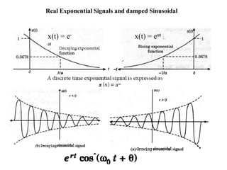
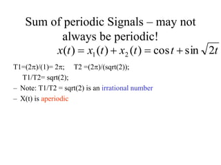
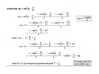
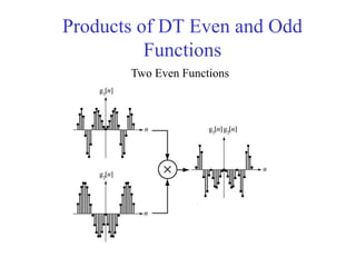
Sinusoidal & Exponential Signals Contd.
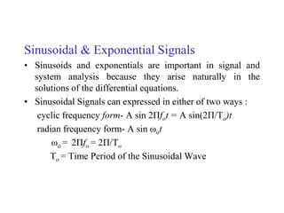
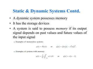
x(t) = A sin (2Пfot+ θ)
= A sin (ωot+ θ)
x(t) = Aeat Real Exponential
= Aejω̥t = A[cos (ωot) +j sin (ωot)] Complex Exponential
θ = Phase of sinusoidal wave
A = amplitude of a sinusoidal or exponential signal
fo = fundamental cyclic frequency of sinusoidal signal
ωo = radian frequency
Sinusoidal signal

x(t) = e-
at
x(t) = eαt
Real Exponential Signals and damped Sinusoidal

Signum Function
   
1 , 0
sgn 0 , 0 2u 1
1 , 0
t
t t t
t
 
 
    
   
Precise Graph Commonly-Used Graph
The signum function, is closely related to the unit-step
function.

Rectangular Pulse or Gate Function
Rectangular pulse,  
1/ , / 2
0 , / 2
a
a t a
t
t a

 
 


The Unit Triangle Function
A triangular pulse whose height and area are both one but its base
width is not, is called unit triangle function. The unit triangle is
related to the unit rectangle through an operation called
convolution.

Sinc Function
 
 sin
sinc
t
t
t




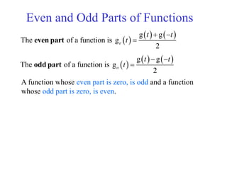
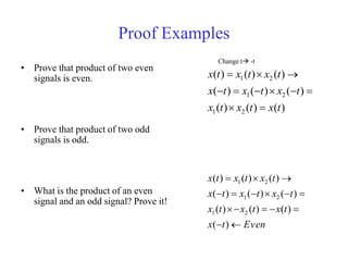
Discrete-Time Signals
• Sampling is the acquisition of the values of a
continuous-time signal at discrete points in time
• x(t) is a continuous-time signal, x[n] is a discrete-
time signal
   x x where is the time between sampless sn nT T

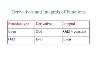
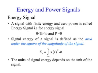
Discrete Time Exponential and
Sinusoidal Signals
• DT signals can be defined in a manner analogous to their
continuous-time counter part
x[n] = A sin (2Пn/No+θ)
= A sin (2ПFon+ θ)
x[n] = an
n = the discrete time
A = amplitude
θ = phase shifting radians,
No = Discrete Period of the wave
1/N0 = Fo = Ωo/2 П = Discrete Frequency
Discrete Time Sinusoidal Signal
Discrete Time Exponential Signal

Discrete Time Sinusoidal Signals

Discrete Time Unit Step Function or
Unit Sequence Function
 
1 , 0
u
0 , 0
n
n
n

 


Discrete Time Unit Ramp Function
   
, 0
ramp u 1
0 , 0
n
m
n n
n m
n 
 
   
 


Discrete Time Unit Impulse Function or
Unit Pulse Sequence
 
1 , 0
0 , 0
n
n
n


 

    for any non-zero, finite integer .n an a 

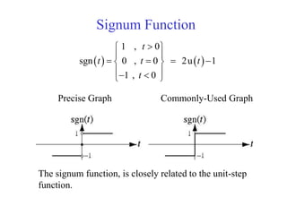
Unit Pulse Sequence Contd.
• The discrete-time unit impulse is a function in the
ordinary sense in contrast with the continuous-
time unit impulse.
• It has a sampling property.
• It has no scaling property i.e.
δ[n]= δ[an] for any non-zero finite integer ‘a’

Operations of Signals
• Sometime a given mathematical function may
completely describe a signal .
• Different operations are required for different
purposes of arbitrary signals.
• The operations on signals can be
Time Shifting
Time Scaling
Time Inversion or Time Folding

Time Shifting
• The original signal x(t) is shifted by an
amount tₒ.
• X(t)X(t-to) Signal Delayed Shift to the
right

Time Shifting Contd.
• X(t)X(t+to) Signal Advanced Shift
to the left

Time Scaling
• For the given function x(t), x(at) is the time
scaled version of x(t)
• For a ˃ 1,period of function x(t) reduces and
function speeds up. Graph of the function
shrinks.
• For a ˂ 1, the period of the x(t) increases
and the function slows down. Graph of the
function expands.

Time scaling Contd.
Example: Given x(t) and we are to find y(t) = x(2t).
The period of x(t) is 2 and the period of y(t) is 1,

Time scaling Contd.
• Given y(t),
– find w(t) = y(3t)
and v(t) = y(t/3).

Time Reversal
• Time reversal is also called time folding
• In Time reversal signal is reversed with
respect to time i.e.
y(t) = x(-t) is obtained for the given
function

0 0, an integern n n n Timeshifting
Operations of Discrete Time
Functions

Operations of Discrete Functions Contd.
Scaling; Signal Compression
n Kn K an integer > 1

Classification of Signals
• Deterministic & Non Deterministic Signals
• Periodic & A periodic Signals
• Even & Odd Signals
• Energy & Power Signals

Deterministic & Non Deterministic Signals
Deterministic signals
• Behavior of these signals is predictable w.r.t time
• There is no uncertainty with respect to its value at any
time.
• These signals can be expressed mathematically.
For example x(t) = sin(3t) is deterministic signal.

Deterministic & Non Deterministic Signals
Contd.
Non Deterministic or Random signals
• Behavior of these signals is random i.e. not predictable
w.r.t time.
• There is an uncertainty with respect to its value at any
time.
• These signals can’t be expressed mathematically.
• For example Thermal Noise generated is non
deterministic signal.

Periodic and Non-periodic Signals
• Given x(t) is a continuous-time signal
• x (t) is periodic iff x(t) = x(t+Tₒ) for any T and any integer n
• Example
– x(t) = A cos(wt)
– x(t+Tₒ) = A cos[wt+Tₒ)] = A cos(wt+wTₒ)= A cos(wt+2)
= A cos(wt)
– Note: Tₒ =1/fₒ ; w2fₒ

Periodic and Non-periodic Signals
Contd.
• For non-periodic signals
x(t) ≠ x(t+Tₒ)
• A non-periodic signal is assumed to have a
period T = ∞
• Example of non periodic signal is an
exponential signal

Important Condition of Periodicity for
Discrete Time Signals
• A discrete time signal is periodic if
x(n) = x(n+N)
• For satisfying the above condition the
frequency of the discrete time signal should
be ratio of two integers
i.e. fₒ = k/N

Sum of periodic Signals
• X(t) = x1(t) + X2(t)
• X(t+T) = x1(t+m1T1) + X2(t+m2T2)
• m1T1=m2T2 = Tₒ = Fundamental period
• Example: cos(t/3)+sin(t/4)
– T1=(2)/(/3)=6; T2 =(2)/(/4)=8;
– T1/T2=6/8 = ¾ = (rational number) = m2/m1
– m1T1=m2T2  Find m1 and m2
– 6.4 = 3.8 = 24 = Tₒ

Sum of periodic Signals – may not
always be periodic!
T1=(2)/(1)= 2; T2 =(2)/(sqrt(2));
T1/T2= sqrt(2);
– Note: T1/T2 = sqrt(2) is an irrational number
– X(t) is aperiodic
tttxtxtx 2sincos)()()( 21 

Even and Odd Signals
Even Functions Odd Functions
g t  g t  g t  g t 

Even and Odd Parts of Functions
 
   g g
The of a function is g
2
e
t t
t
 
even part
 
   g g
The of a function is g
2
o
t t
t
 
odd part
A function whose even part is zero, is odd and a function
whose odd part is zero, is even.

Various Combinations of even and odd
functions
Function type Sum Difference Product Quotient
Both even Even Even Even Even
Both odd Odd Odd Even Even
Even and odd Neither Neither Odd Odd

Derivatives and Integrals of Functions
Function type Derivative Integral
Even Odd Odd + constant
Odd Even Even

Discrete Time Even and Odd Signals
 
   g g
g
2
e
n n
n
 
  
   g g
g
2
o
n n
n
 

   g gn n     g gn n  

Combination of even and odd
function for DT Signals
Function type Sum Difference Product Quotient
Both even Even Even Even Even
Both odd Odd Odd Even Even
Even and odd Even or Odd Even or odd Odd Odd

Products of DT Even and Odd
Functions
Two Even Functions

Functions Contd.
An Even Function and an Odd Function

Proof Examples
• Prove that product of two even
signals is even.
• Prove that product of two odd
signals is odd.
• What is the product of an even
signal and an odd signal? Prove it!
)()()(
)()()(
)()()(
21
21
21
txtxtx
txtxtx
txtxtx



Eventx
txtxtx
txtxtx
txtxtx




)(
)()()(
)()()(
)()()(
21
21
21
Change t -t

Functions Contd.
Two Odd Functions

Energy and Power Signals
Energy Signal
• A signal with finite energy and zero power is called
Energy Signal i.e.for energy signal
0<E<∞ and P =0
• Signal energy of a signal is defined as the area
under the square of the magnitude of the signal.
• The units of signal energy depends on the unit of the
signal.
 
2
x xE t dt


 

Energy and Power Signals Contd.
Power Signal
• Some signals have infinite signal energy. In that
caseit is more convenient to deal with average
signal power.
• For power signals
0<P<∞ and E = ∞
• Average power of the signal is given by
 
/2
2
x
/2
1
lim x
T
T
T
P t dt
T

 

Energy and Power Signals Contd.
• For a periodic signal x(t) the average signal
power is
• T is any period of the signal.
• Periodic signals are generally power signals.
 
2
x
1
x
T
P t dt
T
 

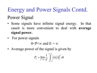
Signal Energy and Power for DT
Signal
•The signal energy of a for a discrete time signal x[n] is
 
2
x x
n
E n


 
•A discrtet time signal with finite energy and zero
power is called Energy Signal i.e.for energy signal
0<E<∞ and P =0

Signal Energy and Power for DT
Signal Contd.
The average signal power of a discrete time power signal
x[n] is
 
1
2
x
1
lim x
2
N
N
n N
P n
N



 
 
2
x
1
x
n N
P n
N 
 
For a periodic signal x[n] the average signal power is
The notation means the sum over any set of
consecutive 's exactly in length.
n N
n N

 
 
 
 


What is System?
• Systems process input signals to produce output
signals
• A system is combination of elements that
manipulates one or more signals to accomplish a
function and produces some output.
system output
signal
input
signal

Types of Systems
• Causal & Anticausal
• Linear & Non Linear
• Time Variant &Time-invariant
• Stable & Unstable
• Static & Dynamic
• Invertible & Inverse Systems

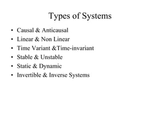
Causal & Anticausal Systems
• Causal system : A system is said to be causal if
the present value of the output signal depends only
on the present and/or past values of the input
signal.
• Example: y[n]=x[n]+1/2x[n-1]

Causal & Anticausal Systems Contd.
• Anticausal system : A system is said to be
anticausal if the present value of the output
signal depends only on the future values of
the input signal.

Time Invariant and Time Variant
Systems
• A system is said to be time invariant if a time
delay or time advance of the input signal leads to a
identical time shift in the output signal.
0
0 0
( ) { ( )}
{ { ( )}} { ( )}
i
t t
y t H x t t
H S x t HS x t
 
 
0
0
0 0
( ) { ( )}
{ { ( )}} { ( )}
t
t t
y t S y t
S H x t S H x t

 

Stable & Unstable Systems
• A system is said to be bounded-input bounded-
output stable (BIBO stable) iff every bounded
input results in a bounded output.
i.e.
| ( )| | ( )|x yt x t M t y t M       

Stable & Unstable Systems Contd.
Example
- y[n]=1/3(x[n]+x[n-1]+x[n-2])
1
[ ] [ ] [ 1] [ 2]
3
1
(| [ ]| | [ 1]| | [ 2]|)
3
1
( )
3
x x x x
y n x n x n x n
x n x n x n
M M M M
    
    
   

Stable & Unstable Systems Contd.
Example: The system represented by
y(t) = A x(t) is unstable ; A˃1
Reason: let us assume x(t) = u(t), then at
every instant u(t) will keep on multiplying
with A and hence it will not be bonded.

Static & Dynamic Systems
• A static system is memoryless system
• It has no storage devices
• its output signal depends on present values of the
input signal
• For example

Static & Dynamic Systems Contd.
• A dynamic system possesses memory
• It has the storage devices
• A system is said to possess memory if its output
signal depends on past values and future values of
the input signal

Invertible & Inverse Systems
• If a system is invertible it has an Inverse System
• Example: y(t)=2x(t)
– System is invertible must have inverse, that is:
– For any x(t) we get a distinct output y(t)
– Thus, the system must have an Inverse
• x(t)=1/2 y(t)=z(t)
y(t)
System
Inverse
System
x(t) x(t)
y(t)=2x(t)System
(multiplier)
Inverse
System
(divider)
x(t) x(t)

Discrete-Time Systems
• A Discrete-Time System is a mathematical operation that
maps a given input sequence x[n] into an output sequence
y[n]
Example:
Moving (Running) Average
Maximum
Ideal Delay System
]}n[x{T]n[y 
]3n[x]2n[x]1n[x]n[x]n[y 
 ]2n[x],1n[x],n[xmax]n[y 
]nn[x]n[y o

Memoryless System
A system is memoryless if the output y[n] at every value
of n depends only on the input x[n] at the same value of n
Example :
Square
Sign
counter example:
Ideal Delay System
 2
]n[x]n[y 
 ]n[xsign]n[y 
]nn[x]n[y o

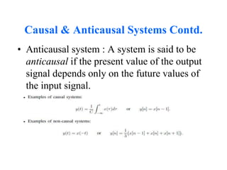
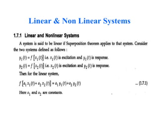
Linear Systems
• Linear System: A system is linear if and only if
Example: Ideal Delay System
   
    (scaling)]n[xaT]n[axT
and
y)(additivit]n[xT]n[xT]}n[x]n[x{T 2121


]nn[x]n[y o
 
 
  ]nn[ax]n[xaT
]nn[ax]n[axT
]nn[x]nn[x]n[xT]}n[x{T
]nn[x]nn[x]}n[x]n[x{T
o1
o1
o2o112
o2o121





Time-Invariant Systems
Time-Invariant (shift-invariant) Systems
A time shift at the input causes corresponding time-shift at
output
Example: Square
Counter Example: Compressor System
 ]nn[xT]nn[y]}n[x{T]n[y oo 
 2
]n[x]n[y 
   
   2
oo
2
o1
]nn[xn-nygivesoutputtheDelay
]nn[xnyisoutputtheinputtheDelay


]Mn[x]n[y 
 
    oo
o1
nnMxn-nygivesoutputtheDelay
]nMn[xnyisoutputtheinputtheDelay



Causal System
A system is causal iff it’s output is a function of only the
current and previous samples
Examples: Backward Difference
Counter Example: Forward Difference
]n[x]1n[x]n[y 
]1n[x]n[x]n[y 

Stable System
Stability (in the sense of bounded-input bounded-output
BIBO). A system is stable iff every bounded input produces
a bounded output
Example: Square
Counter Example: Log
 yx B]n[yB]n[x
 2
]n[x]n[y 


2
x
x
B]n[ybyboundedisoutput
B]n[xbyboundedisinputif
 ]n[xlog]n[y 10
       

nxlog0y0nxforboundednotoutput
B]n[xbyboundedisinputifeven
10
x

Classification of-signals-systems-ppt

More Related Content

What's hot

Similar to Classification of-signals-systems-ppt

Recently uploaded

Classification of-signals-systems-ppt