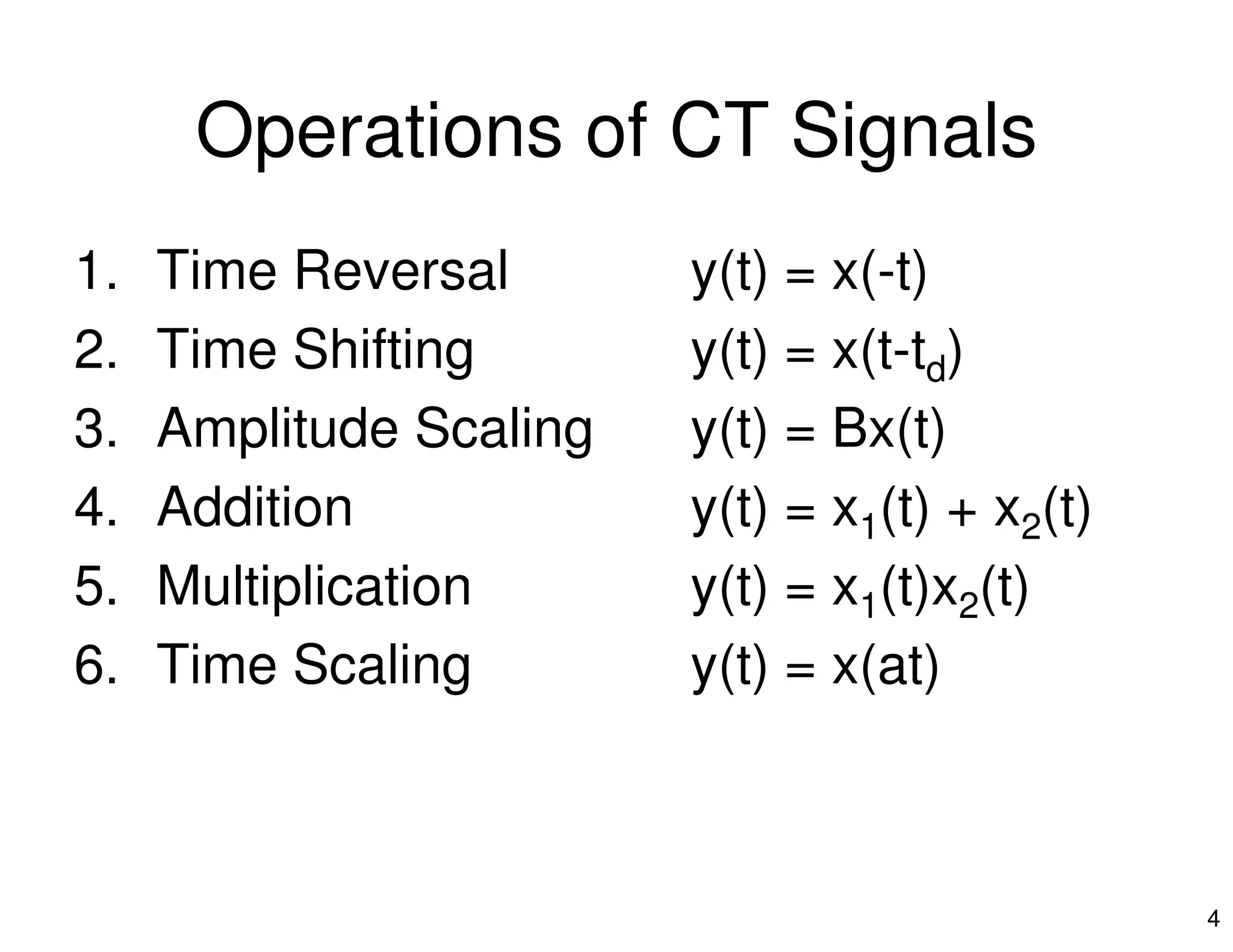
1. The document discusses operations that can be performed on continuous-time signals, including time reversal, time shifting, amplitude scaling, addition, multiplication, and time scaling.
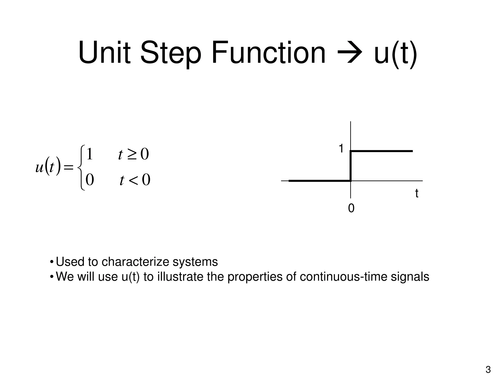
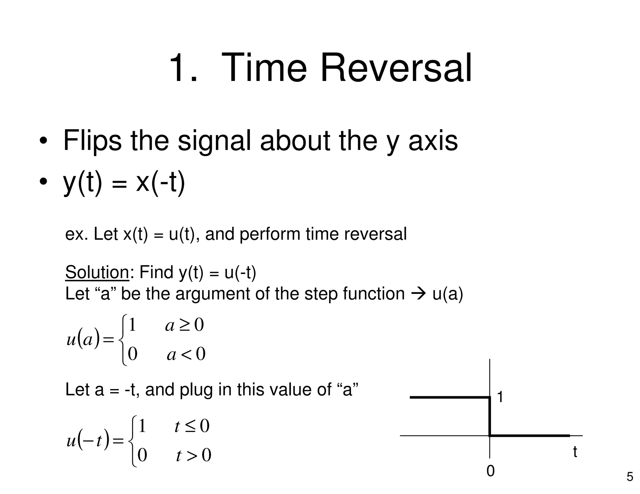
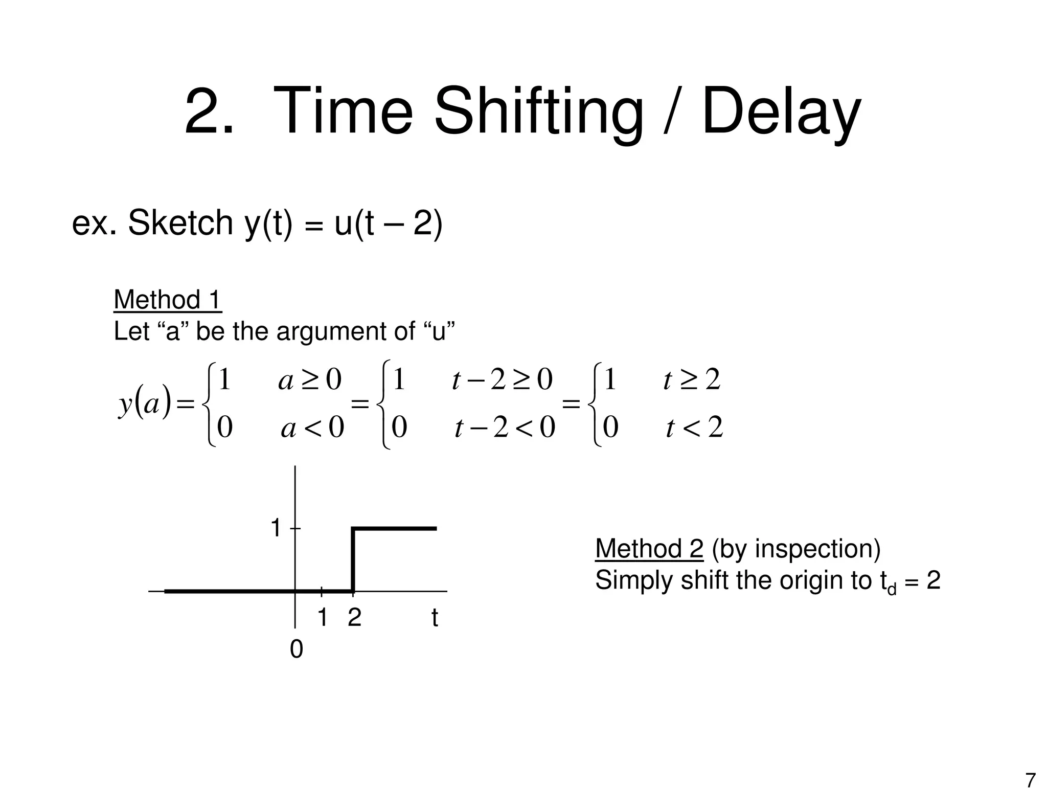
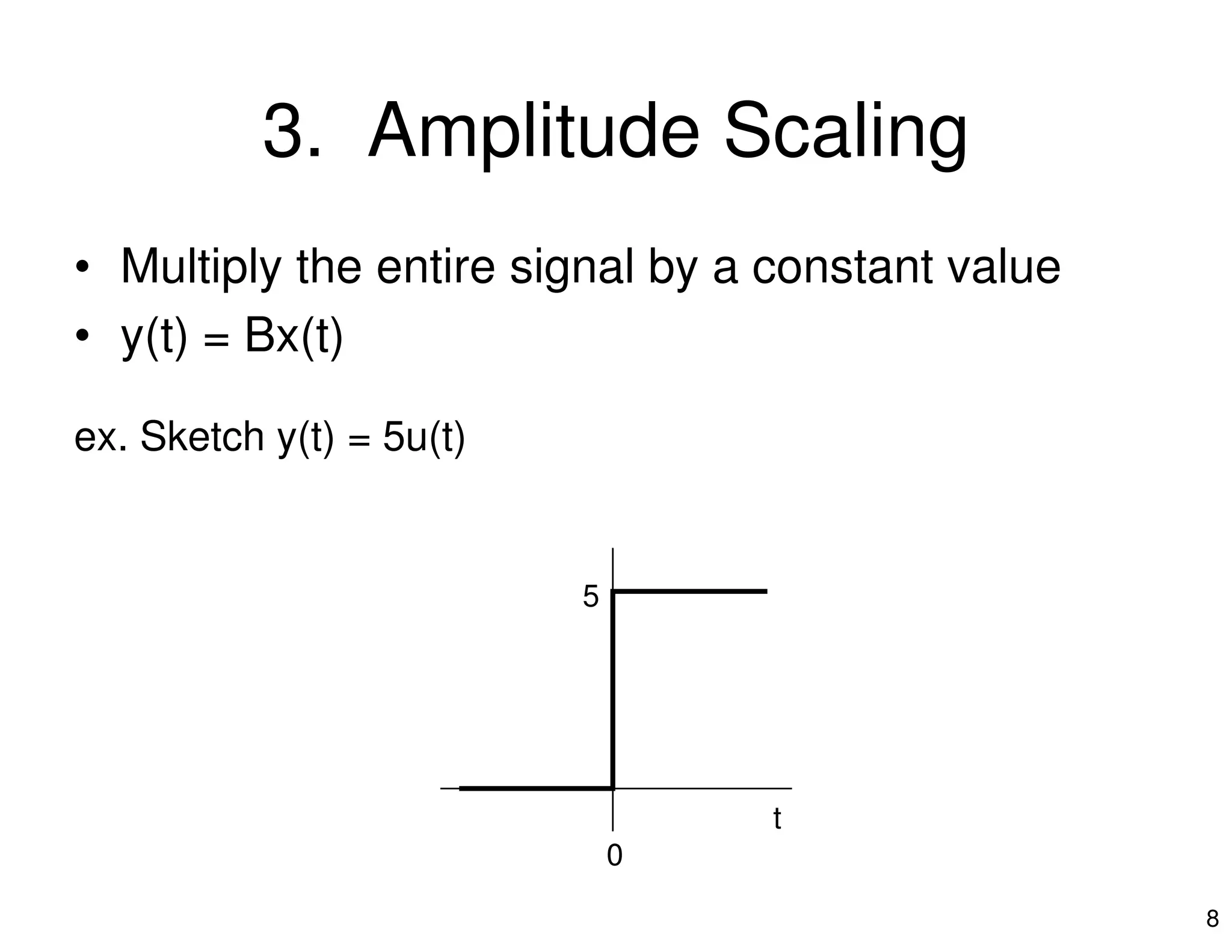
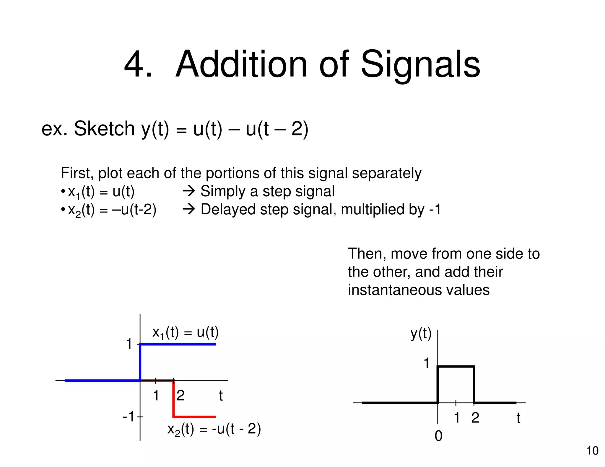
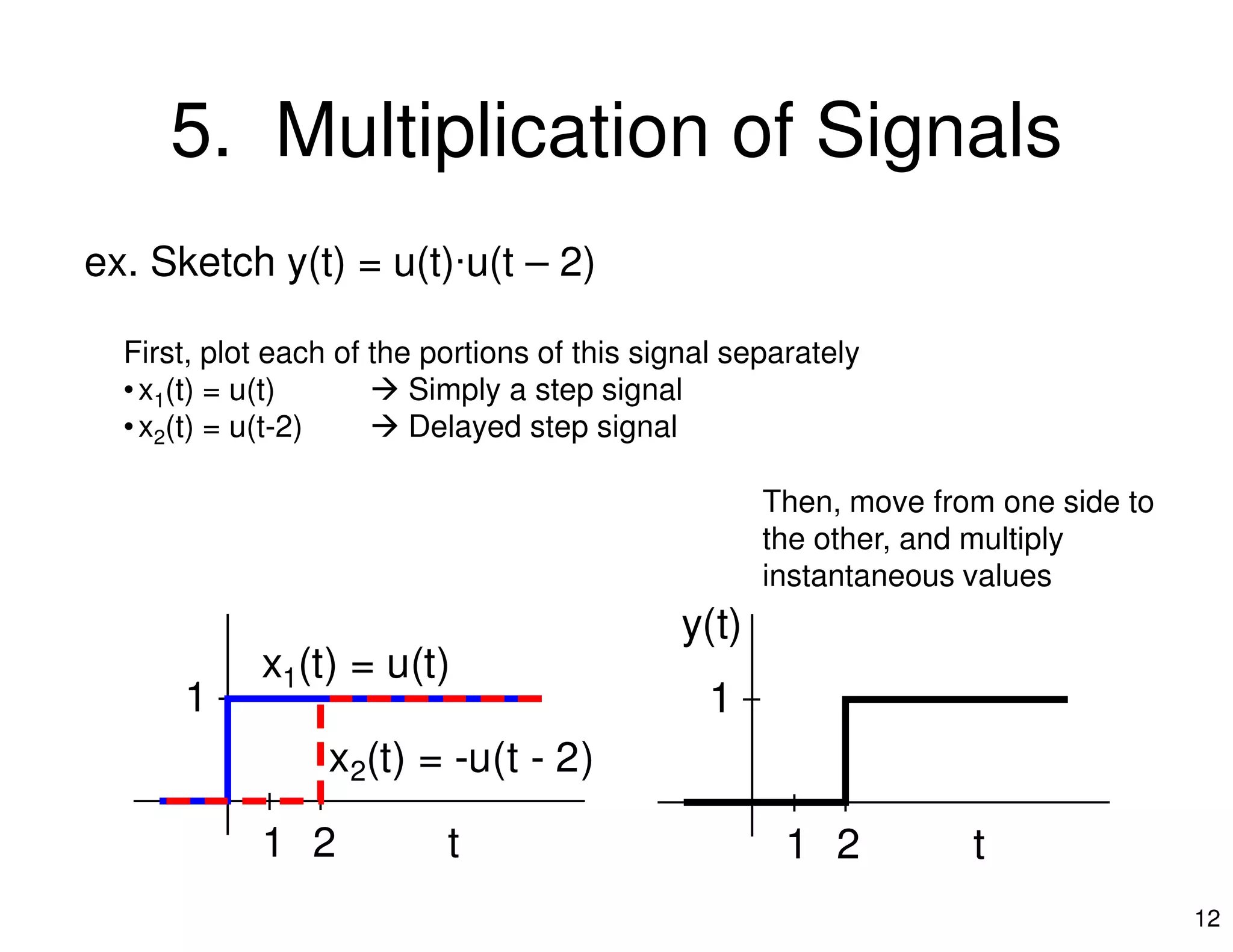
2. It provides examples of each operation using the unit step function u(t) and illustrates the effect graphically. Combinations of operations are also demonstrated through examples.
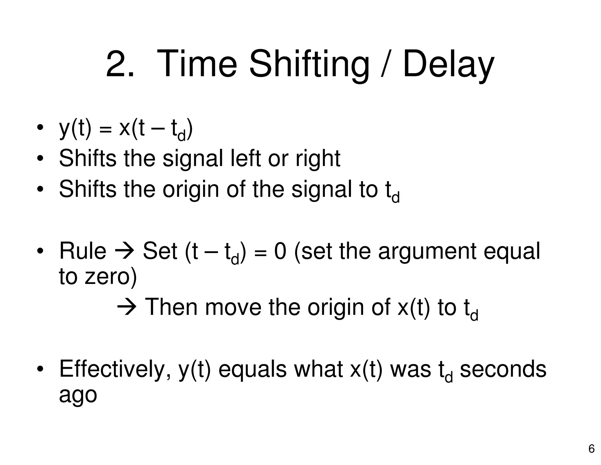
3. Key operations include time shifting which delays a signal, time scaling which speeds up or slows down a signal, and their combination which first performs one operation and then the other.
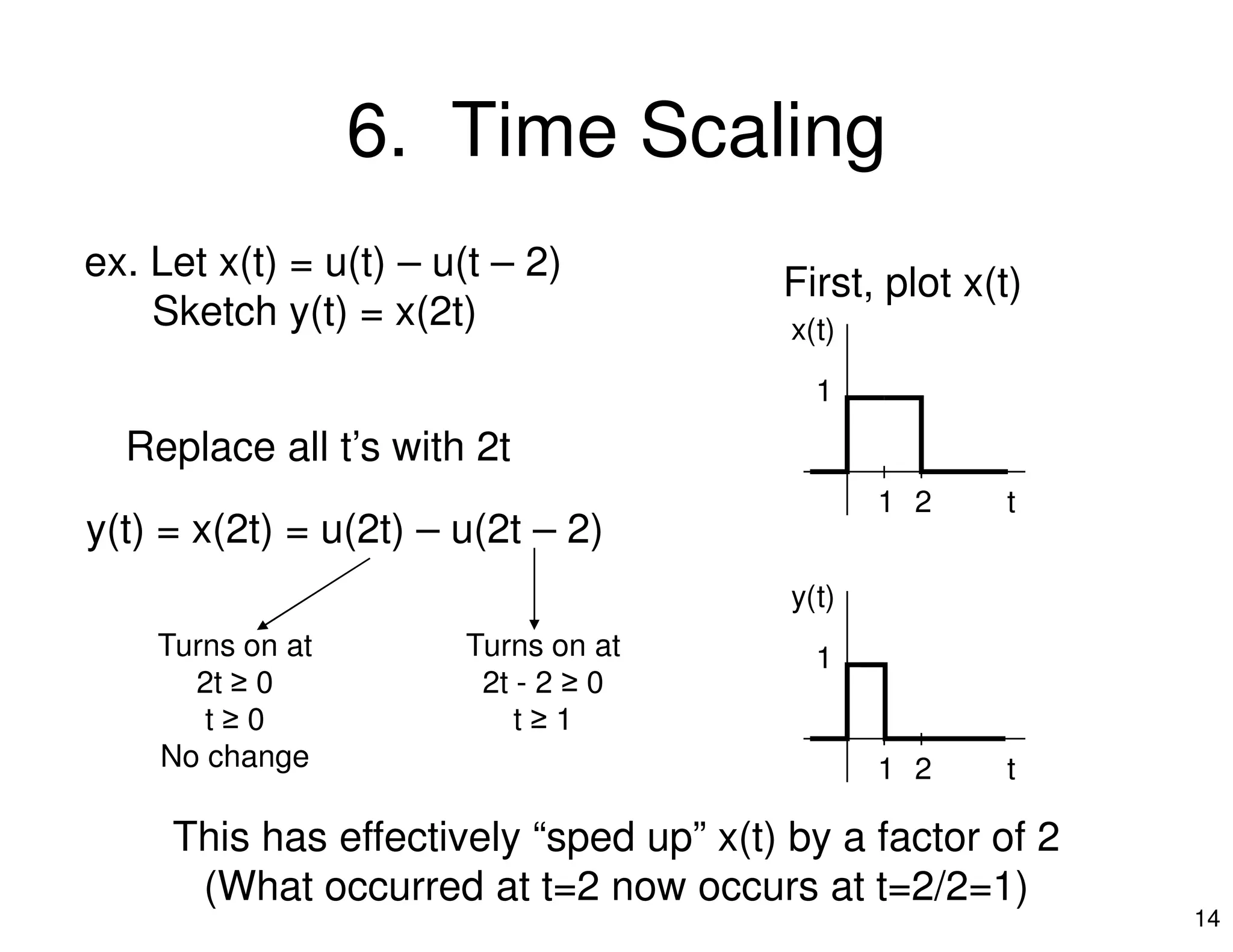
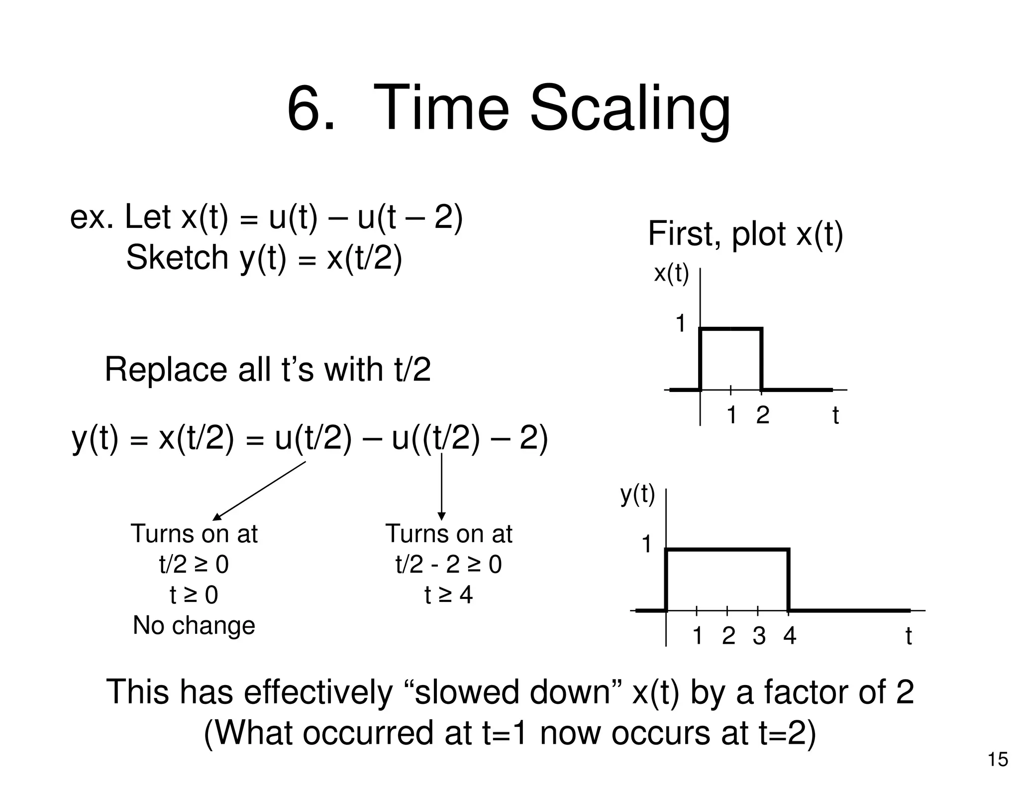
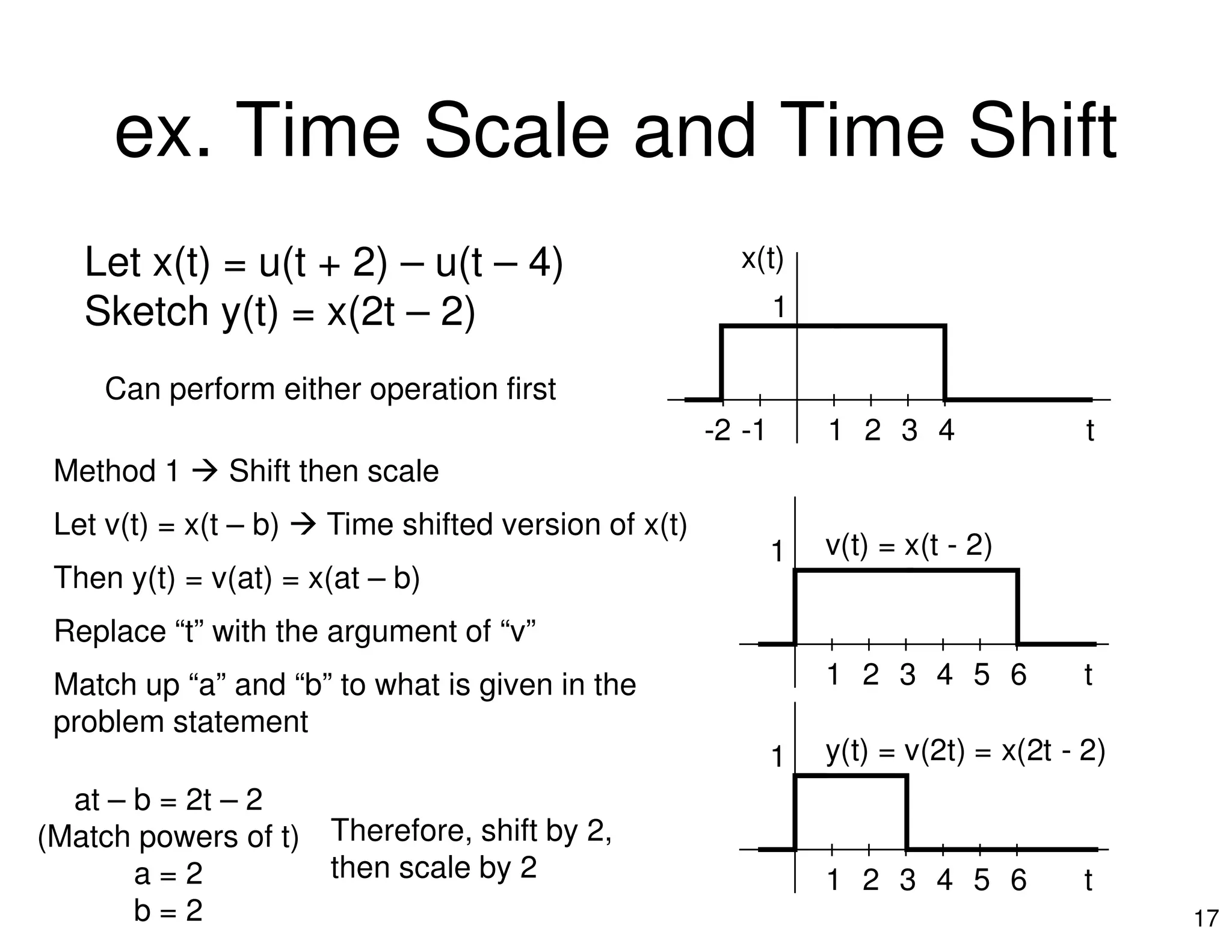
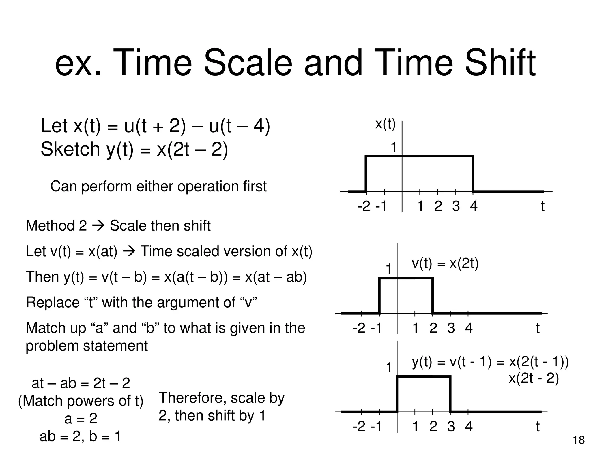
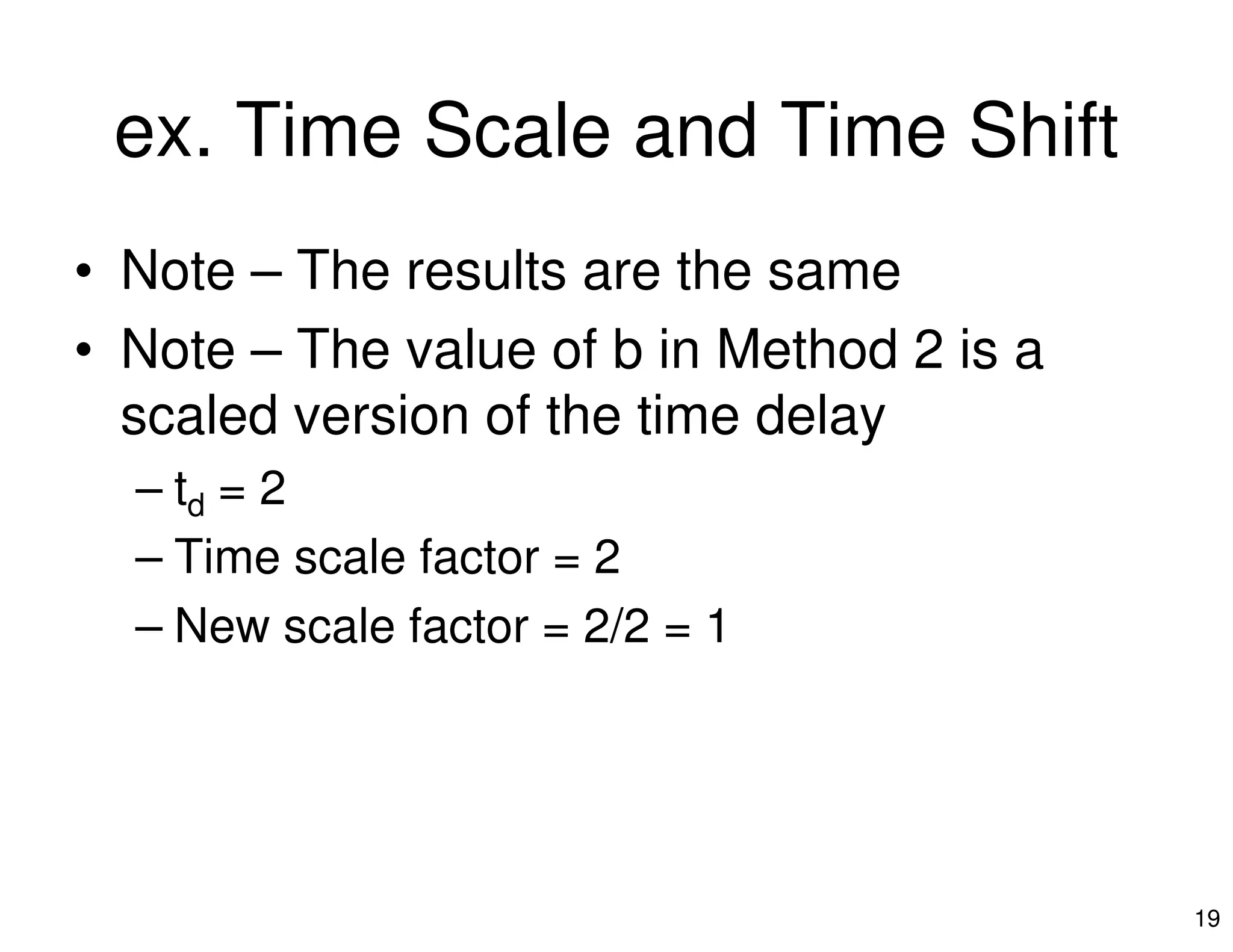


![Circuit Network Analysis - [Chapter4] Laplace Transform](https://cdn.slidesharecdn.com/ss_thumbnails/ch4-150613063858-lva1-app6891-thumbnail.jpg?width=640&height=640&fit=bounds)