Downloaded 22 times
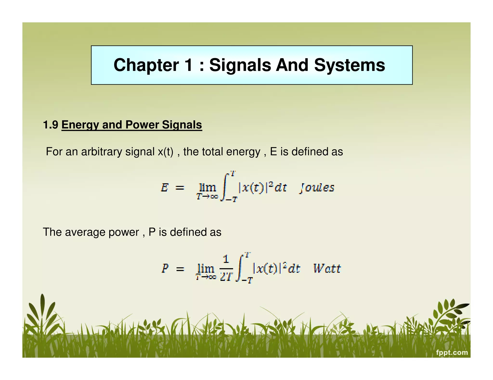

![Chapter 1 : Signals And Systems
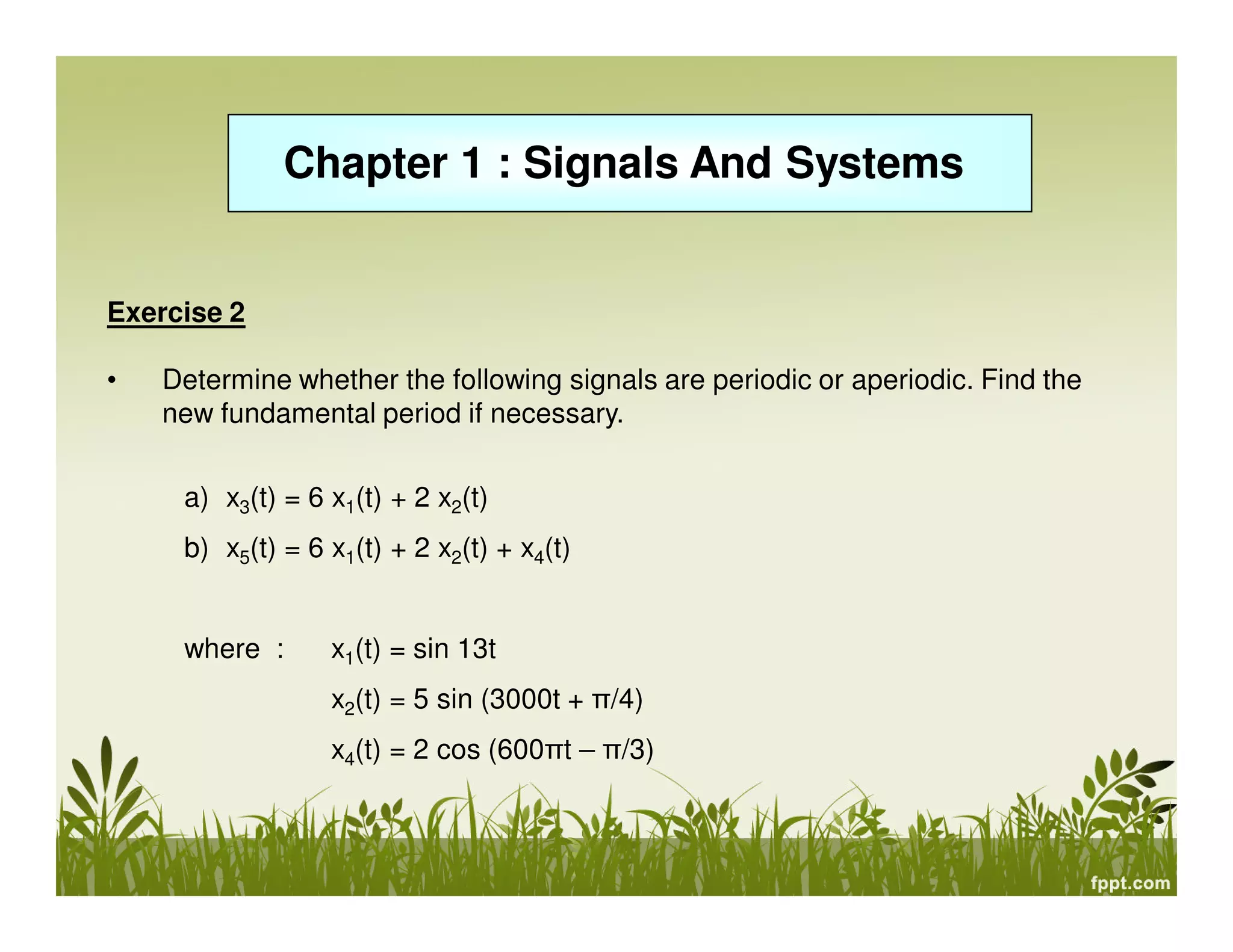
Exercise 1
• Determine whether listed x(t) below is periodic or aperiodic signal. If a signal is
periodic, determine its fundamental period.
a) x(t) = sin 3t
b) x(t) = 2 cos 8πt
c) x(t) = 3 cos (5πt + π/2)
d) x(t) = cos t + sin √2 t
e) x(t) = sin2
t
f) x(t) = e
j[(π/2)t-1]
0
2
ω
π
=T](https://image.slidesharecdn.com/signalsandsystemschapter1-131124023113-phpapp01-150917214129-lva1-app6891/75/Signals-and-system-21-2048.jpg)
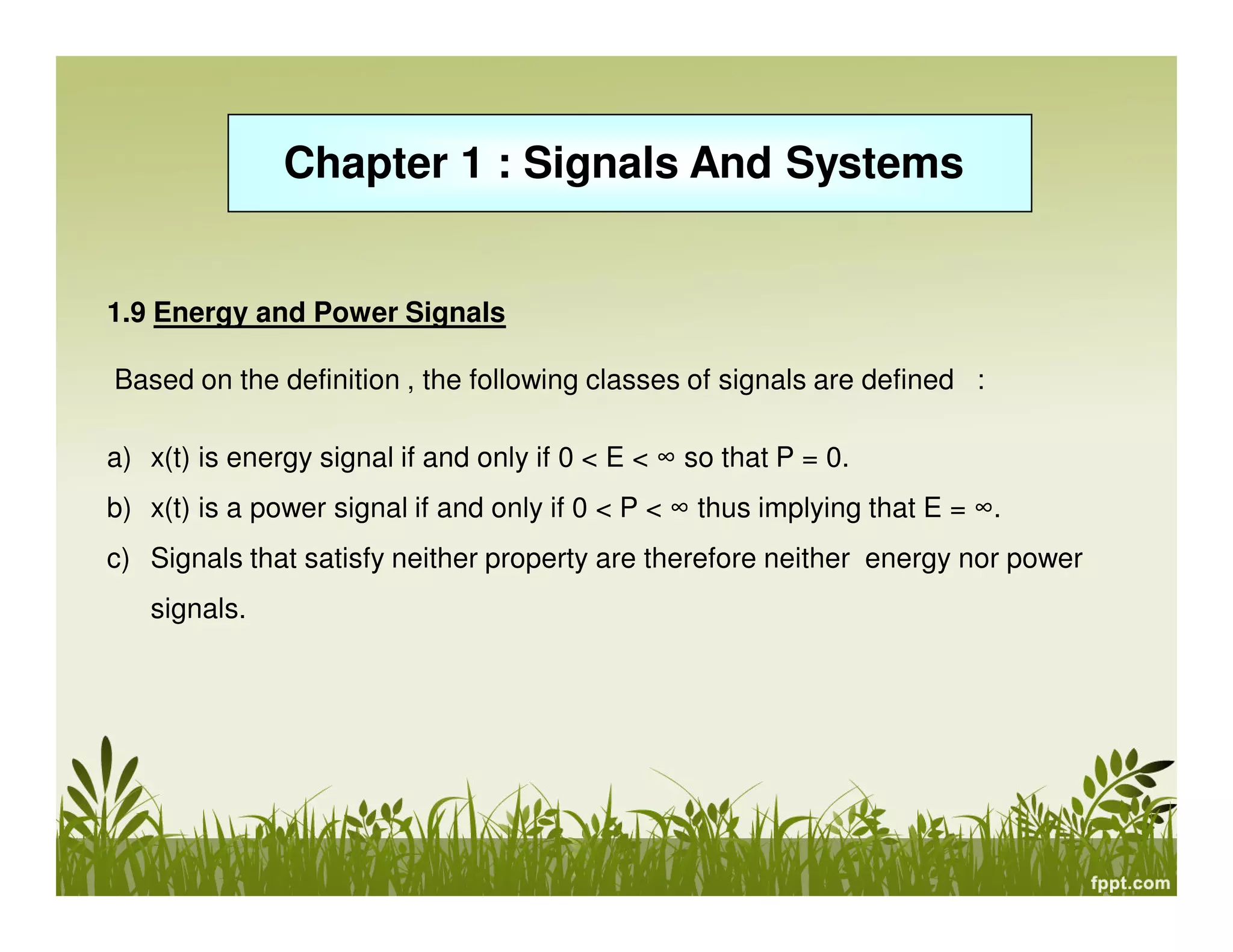
![EXERCISE 2
a) x[n]=e
j(π/4)n
b) x[n]=cos1/4n
c) x[n]= cos π/3 n + sin π/4n
d) x[n]=cos2π/8n](https://image.slidesharecdn.com/signalsandsystemschapter1-131124023113-phpapp01-150917214129-lva1-app6891/75/Signals-and-system-22-2048.jpg)

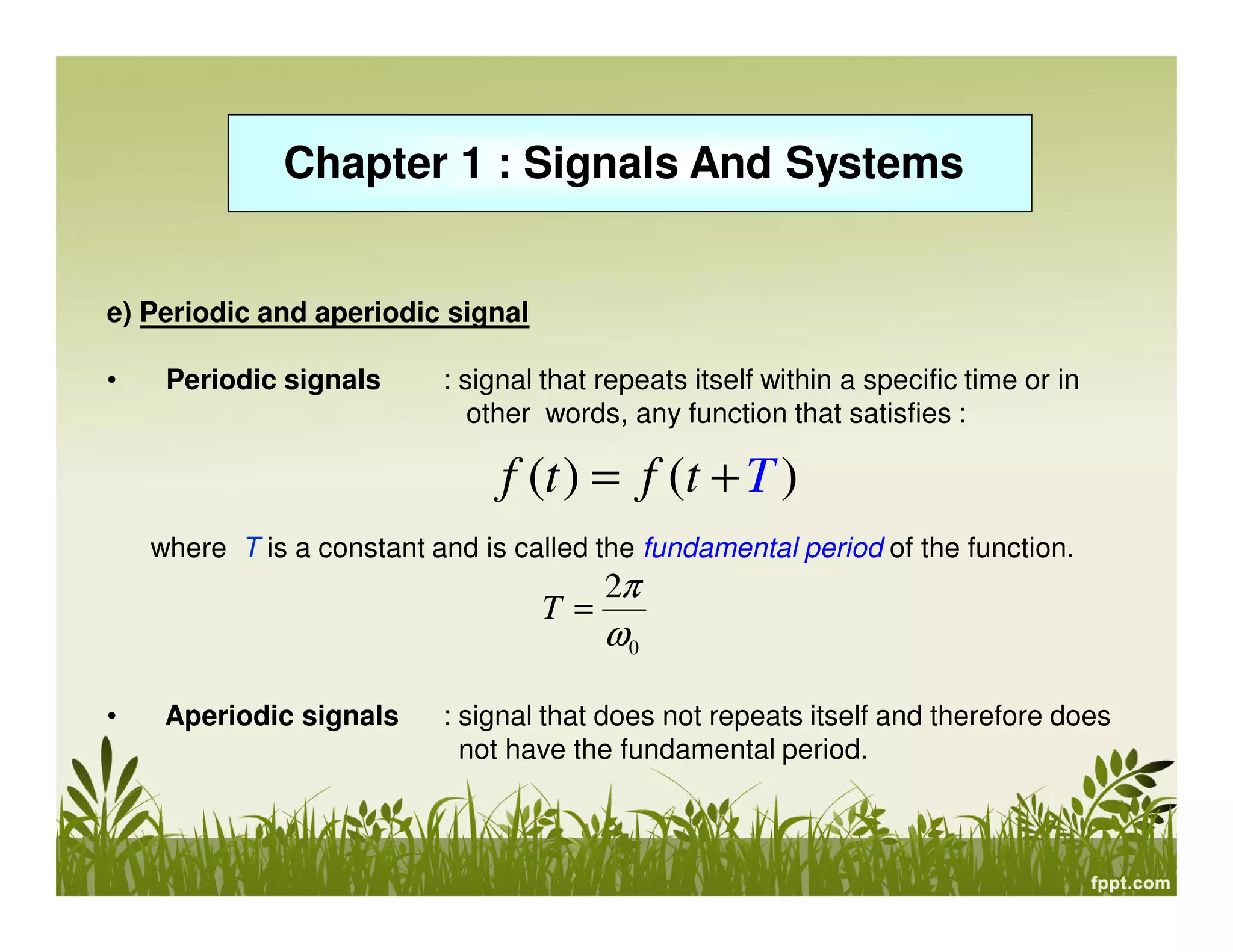
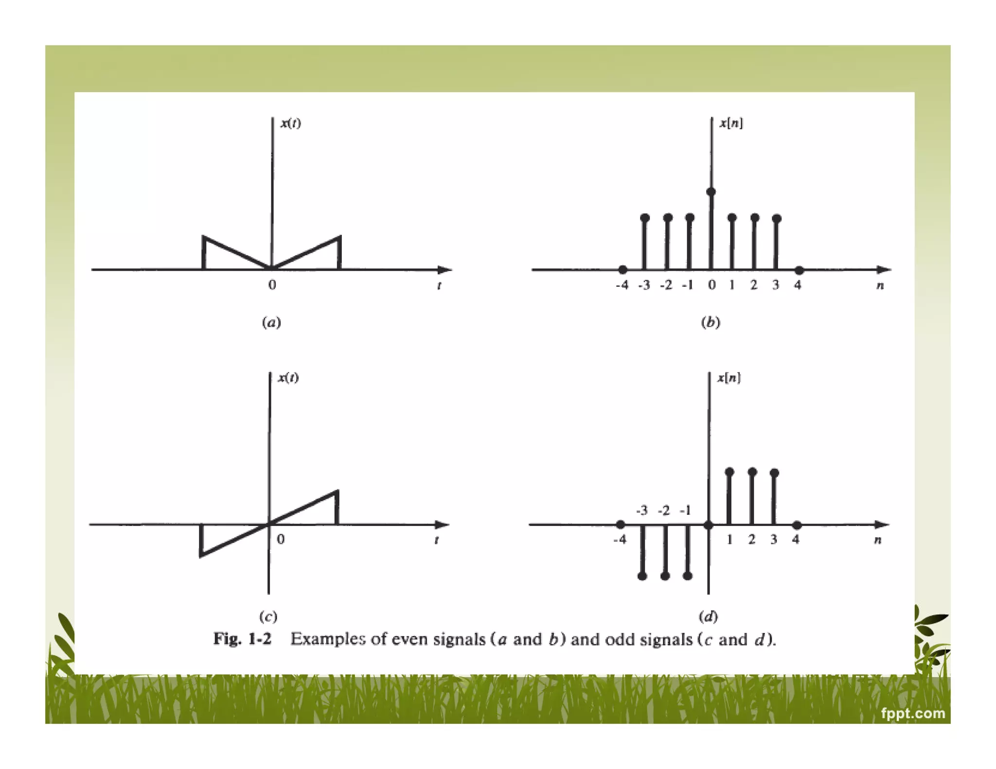
![• Even and Odd
A signal x ( t ) or x[n] is referred to as an even signal if
x ( - t ) = x ( r )
x [ - n ] = x [ n ]
A signal x ( t ) or x[n] is referred to as an odd signal if
x ( - t ) = - x ( t )
x [ - n ] = - x [ n ]
Examples of even and odd signals are shown in Fig. 1-2.
Chapter 1 : Signals And Systems](https://image.slidesharecdn.com/signalsandsystemschapter1-131124023113-phpapp01-150917214129-lva1-app6891/75/Signals-and-system-25-2048.jpg)


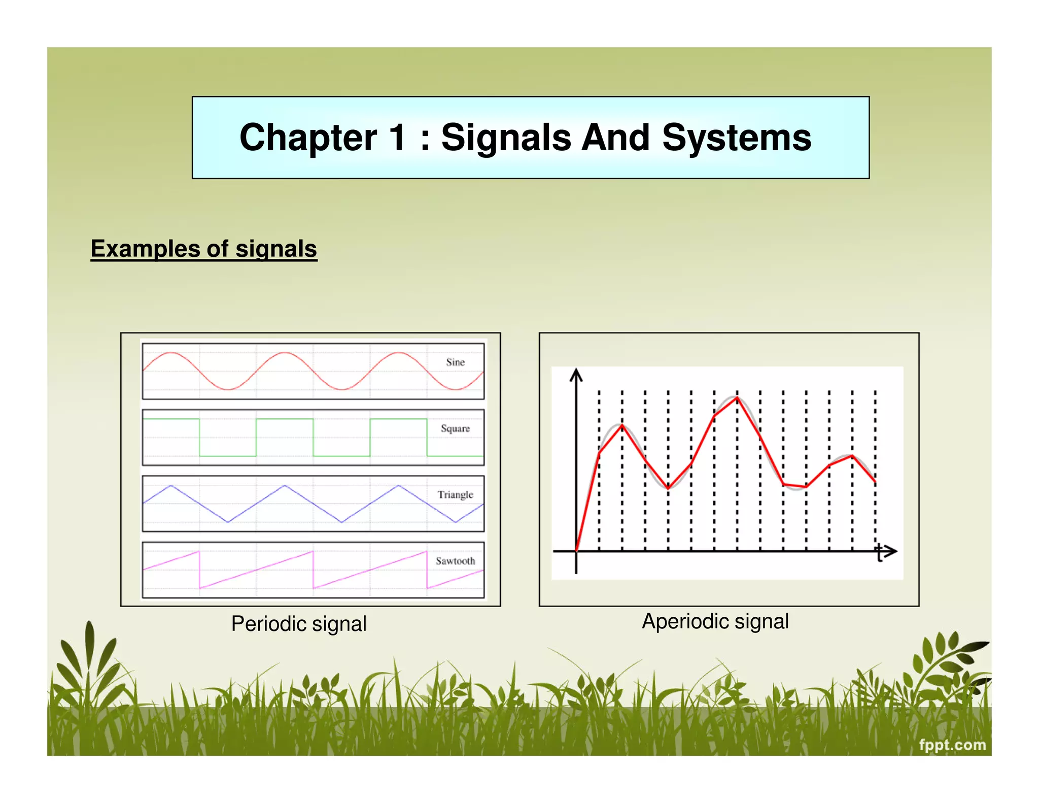
![Chapter 1 : Signals And Systems
2.0 Classification Of System
4) a) Linear : y(t) = ay1(t) + by2(t) (superposition applied)
b) Non linear : y(t) ≠ ay1(t) + by2(t) (superposition not applied )
where :
If an excitation x1[t] causes a response y1[t] and an excitation x2 [t] causes a
response y2[n] , then an excitation :
x [t = ax1[t] + bx2[t] (to be presented as y(t) in solution)
y [t] = ay1[t] + by2[t]
will cause the response](https://image.slidesharecdn.com/signalsandsystemschapter1-131124023113-phpapp01-150917214129-lva1-app6891/75/Signals-and-system-50-2048.jpg)


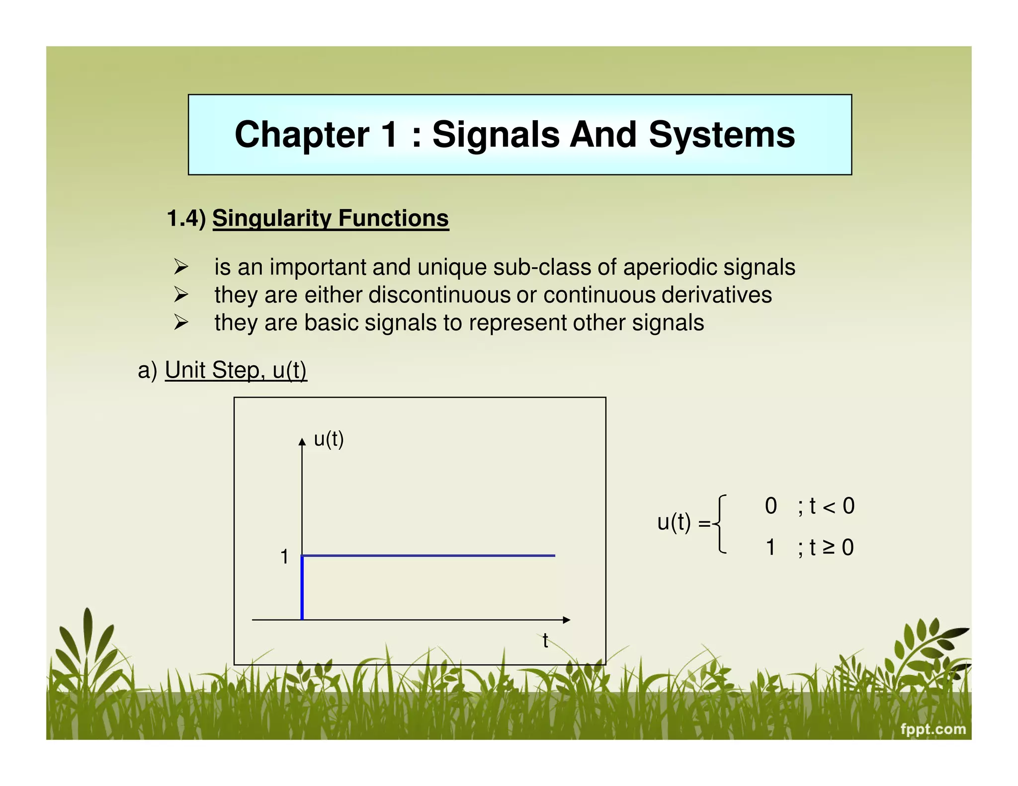
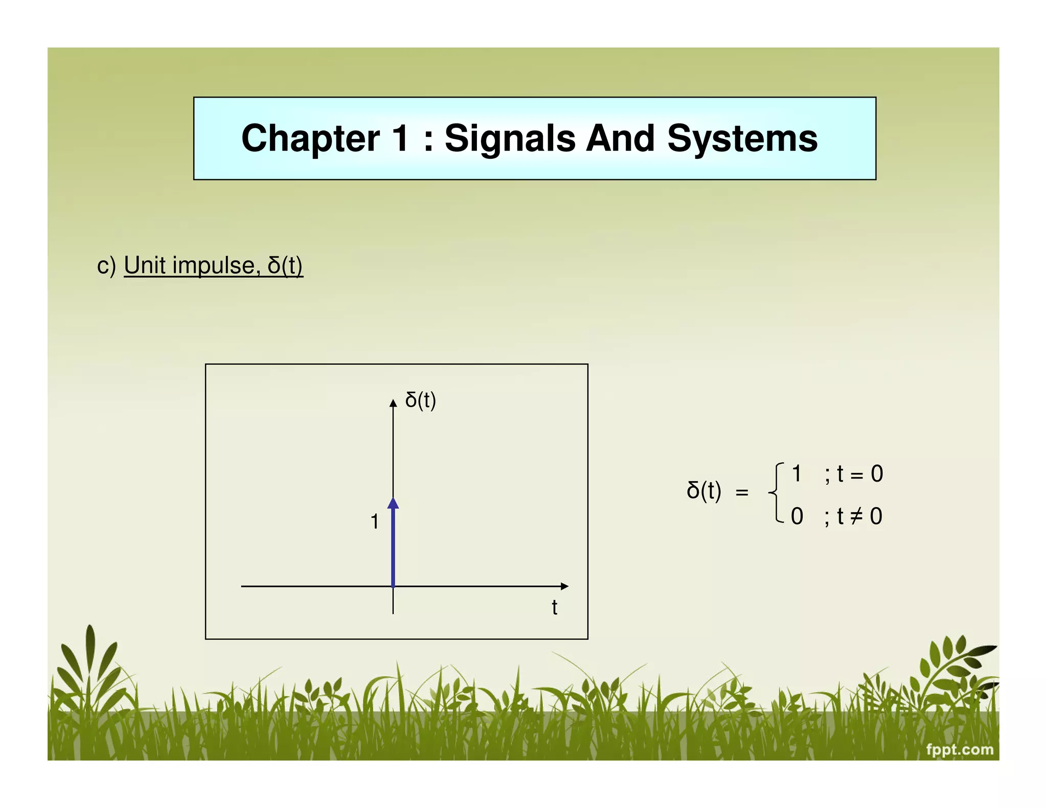
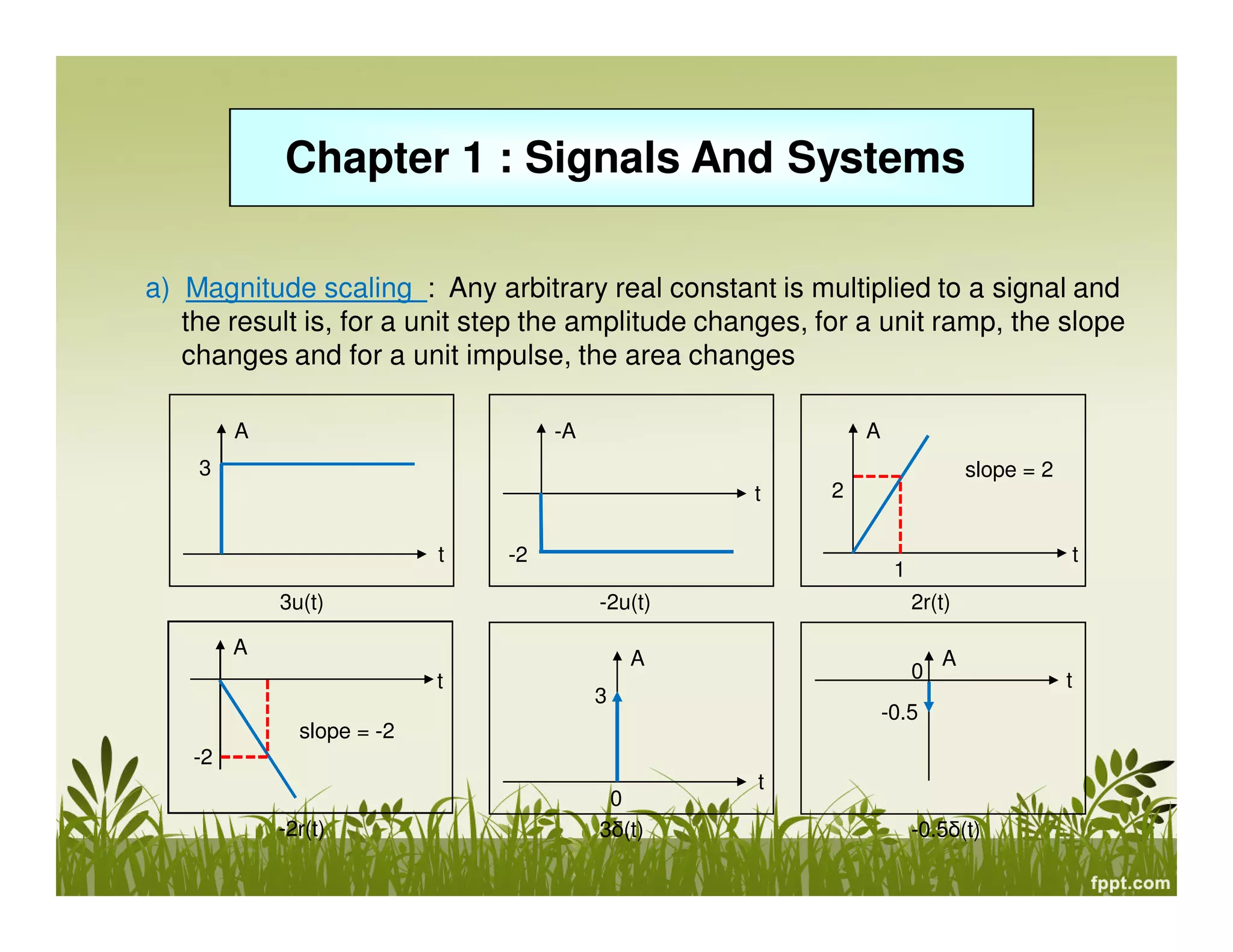
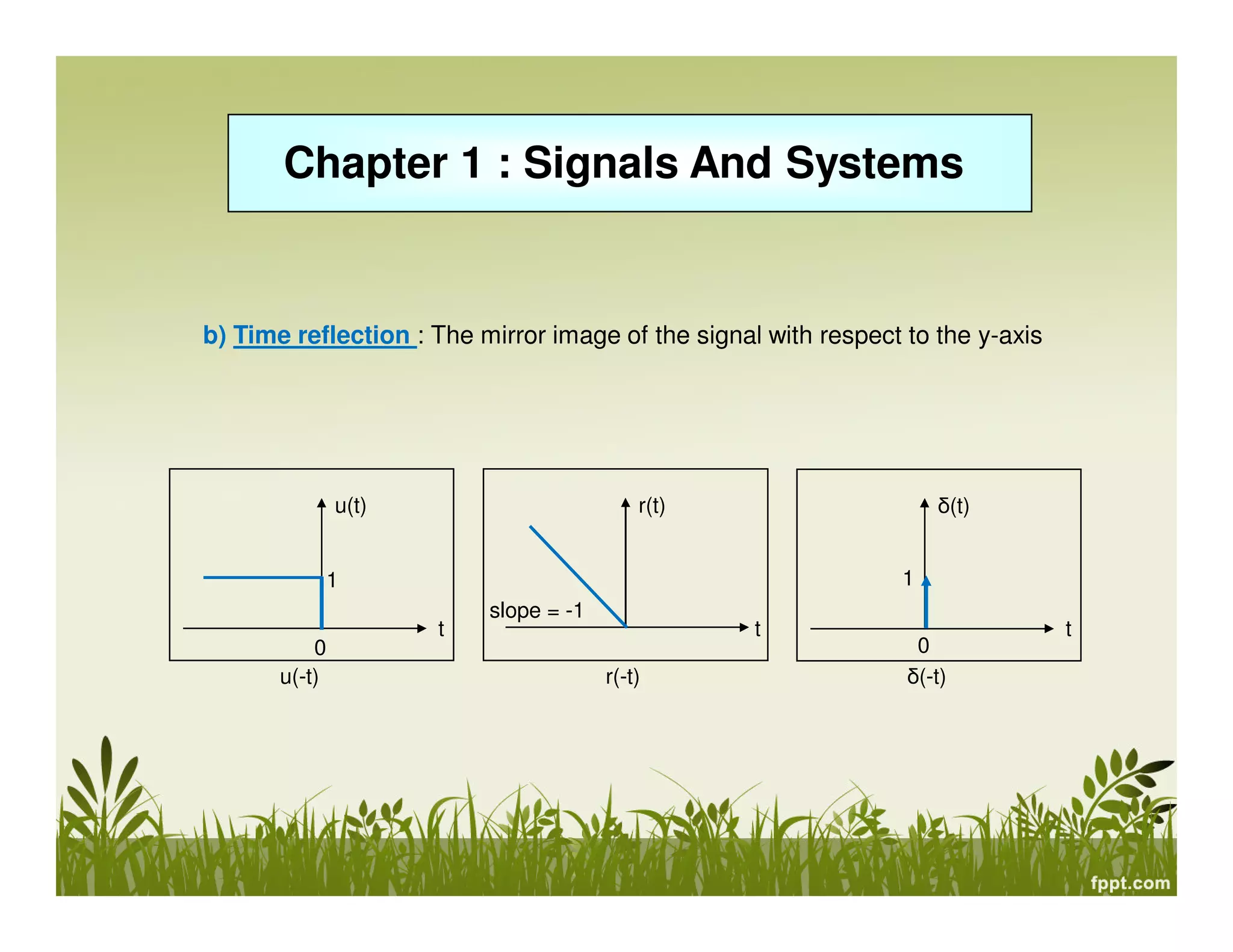
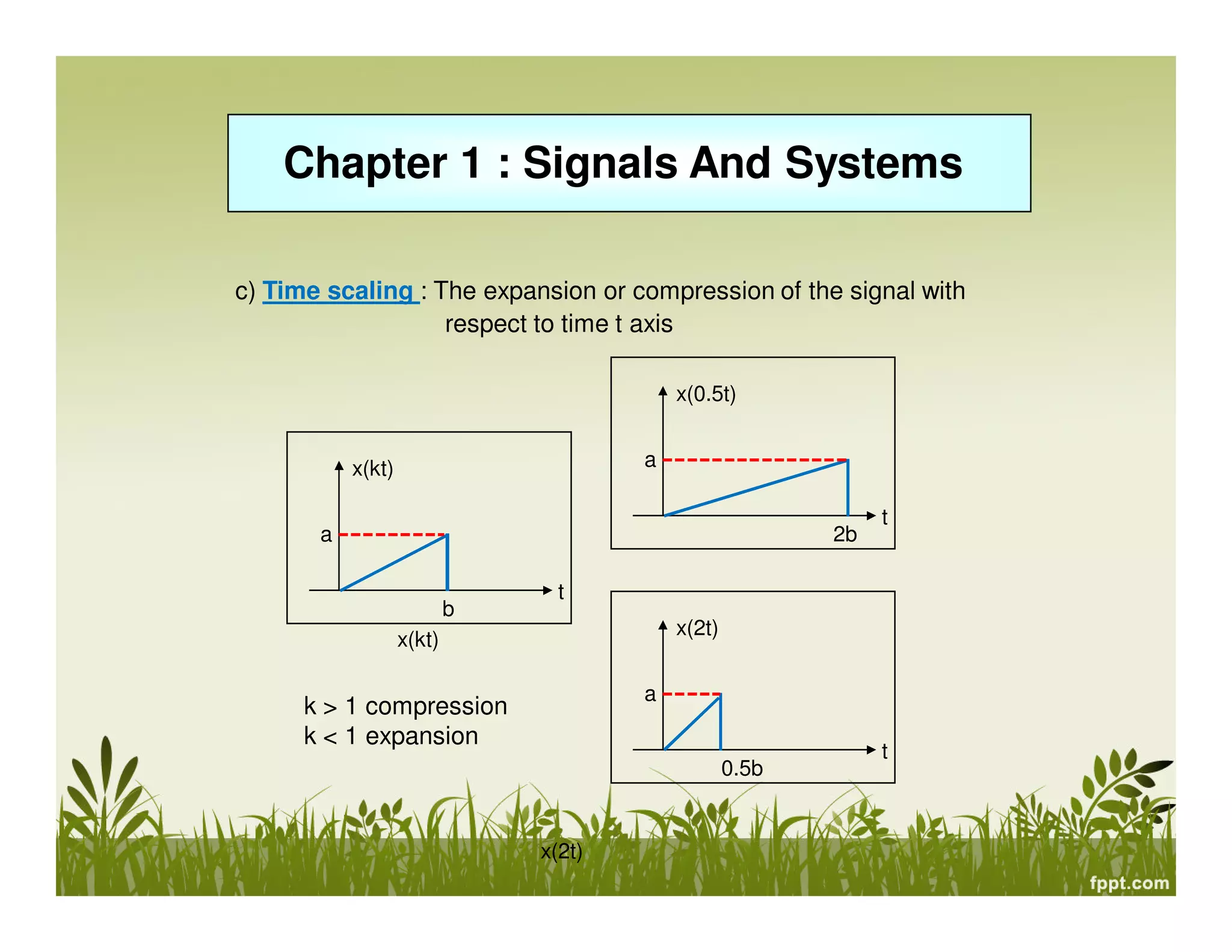
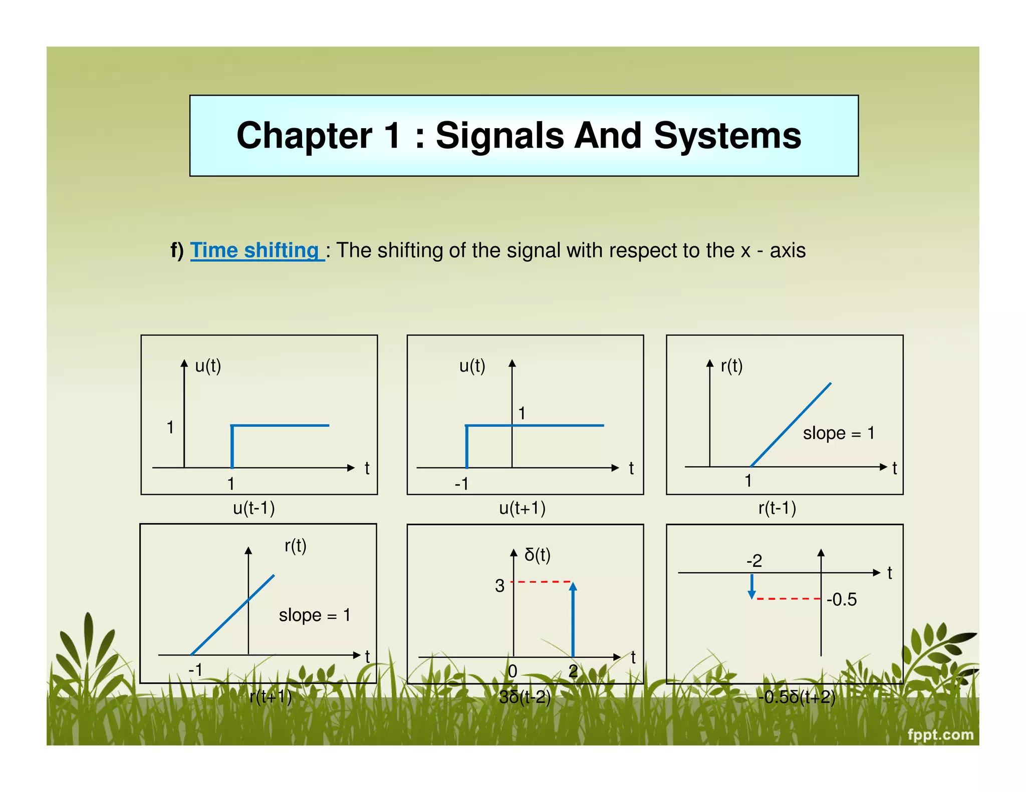
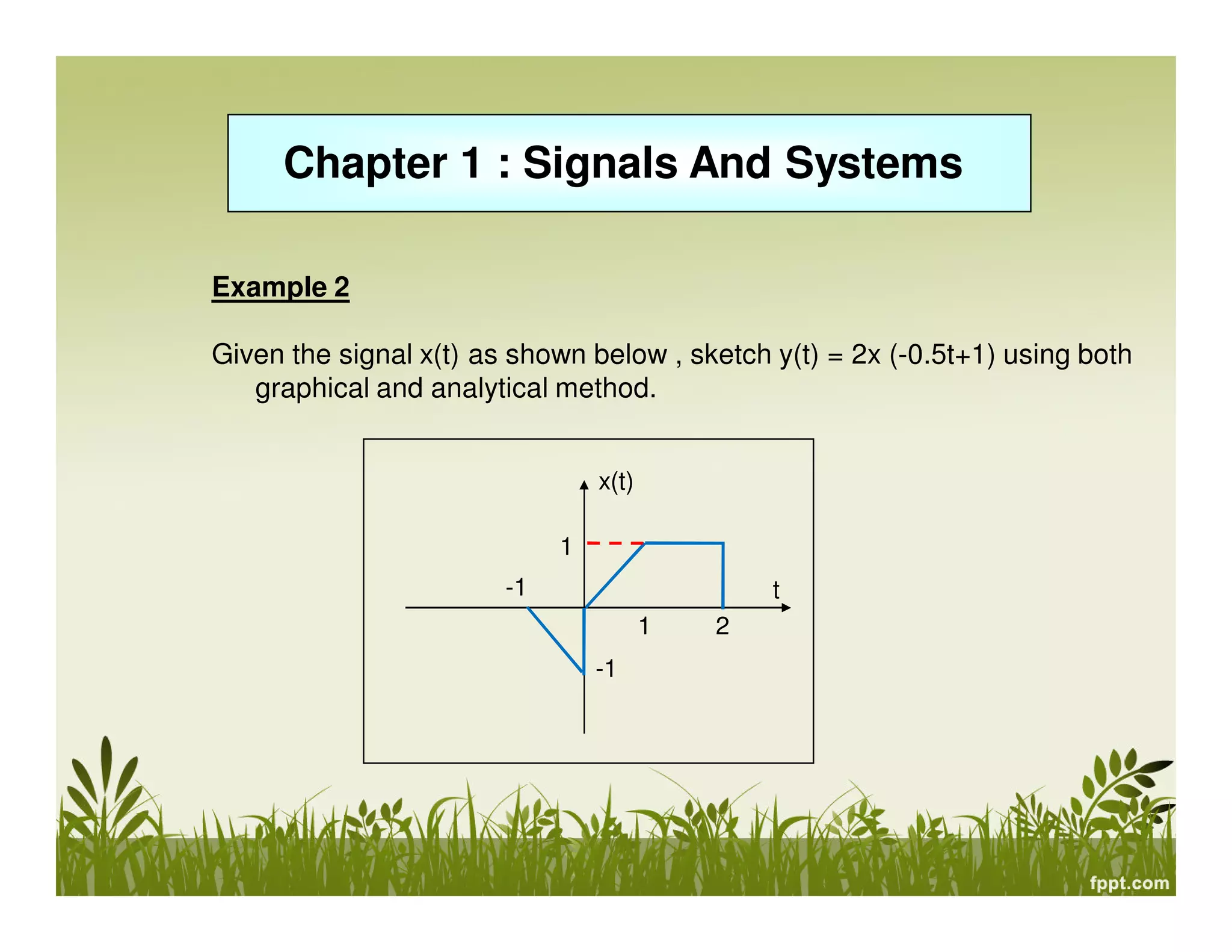
This document provides an overview of signals and systems. It defines key terms like signals, systems, continuous and discrete time signals, analog and digital signals, deterministic and probabilistic signals, even and odd signals, energy and power signals, periodic and aperiodic signals. It also classifies systems as linear/non-linear, time-invariant/variant, causal/non-causal, and with or without memory. Singularity functions like unit step, unit ramp and unit impulse are introduced. Properties of signals like magnitude scaling, time reflection, time scaling and time shifting are discussed. Energy and power of signals are defined.


![ANPARA THERMAL POWER STATION[1] sangam.pdf](https://cdn.slidesharecdn.com/ss_thumbnails/anparathermalpowerstation1sangam-251121115219-9261cde4-thumbnail.jpg?width=640&height=640&fit=bounds)


