The document discusses the Discrete-Time Fourier Transform (DTFT), its properties, convergence conditions, and the application of Fourier analysis in image processing. It explores the DTFT's role in transforming sequences into the frequency domain, enabling efficient filtering and analysis of signals. Key concepts include magnitude and phase spectra, mean-square convergence, and the Gibbs phenomenon.

1. Discrete Time Fourier Transform
• Why Fourier Transform
• General Properties & Symmetry relations
• Formula and steps
• magnitude and phase spectra
• Convergence Condition
• mean-square convergence
• Gibbs phenomenon
• Direct Delta
• Energy Density Spectrum

2. Image Transforms
• Many times, image processing tasks can be
best performed in a domain other than the
spatial domain.
• Key steps
(1) Transform the image
(2) Carry the task(s) in the transformed domain.
(3) Apply inverse transform to return to the
spatial domain.

3. Why is FT Useful?
• Easier to remove undesirable frequencies in
the frequency domain.
• Faster to perform certain operations in the
frequency domain than in the spatial domain.
– i.e., using the Fast Fourier Transform (FFT)

4. Frequency Filtering: Main Steps
1. Take the FT of f(x):
2. Remove undesired frequencies:
3. Convert back to a signal:
x

5. Example: Removing undesirable frequencies
remove high
frequencies
filtered
signal
frequencies
noisy signal

6. FT - Definitions
• F(u) is a complex function:
• Magnitude of FT (or spectrum):
• Phase of FT:
• Magnitude-Phase representation:
• Power of f(x): P(u)=|F(u)|2=

7. Discrete-Time Fourier Transform
• Definition - The Discrete-Time Fourier
Transform (DTFT) of a sequence
x[n] is given by
• In general, is a complex function of
the real variable w and can be written as
)
( w
j
e
X
)
( w
j
e
X






n
n
j
j
e
n
x
e
X ω
ω
]
[
)
(
)
(
)
(
)
( im
re
w
w
w j
j
j
e
X
j
e
X
e
X 


8. Discrete-Time Fourier Transform
• and are, respectively, the
real and imaginary parts of , and are
real functions of w
• can alternately be expressed as
where
)
( w
j
e
X
)
( ω
re
j
e
X )
( ω
im
j
e
X
)
( w
j
e
X
)
(
)
(
)
( w

w
w  j
j
j e
e
X
e
X
)}
(
arg{
)
( w

w
 j
e
X

9. Discrete-Time Fourier Transform
• is called the magnitude function
• is called the phase function
• Both quantities are again real functions of w
• In many applications, the DTFT is called the
Fourier spectrum
• Likewise, and are called the
magnitude and phase spectra
)
( w
j
e
X
)
(w

)
( w
j
e
X )
(w


10. Discrete-Time Fourier Transform
• Inverse Discrete-Time Fourier Transform:
 w





w
w
d
e
e
X
n
x n
j
j
)
(
2
1
]
[

11. General Properties of DTFT

12. Symmetry relations of the DTFT of a
complex sequence

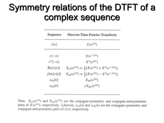
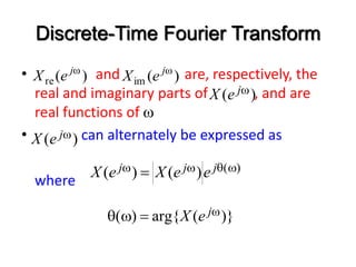
13. Symmetry relations of the DTFT
of a real sequence
x[n]: A real sequence

14. DTFT of unit Impulse Sequence
• Example - The DTFT of the unit sample
sequence d[n] is given by
1
]
0
[
]
[
)
( 
d

d

w
 w




n
j
n
e
n






n
n
j
j
e
n
x
e
X ω
ω
]
[
)
(

15. DTFT of Causal Sequence
• Example - Consider the causal sequence


 



otherwise
0
0
1
]
[
,
1
],
[
]
[
n
n
n
n
x n










n
n
j
j
e
n
x
e
X ω
ω
]
[
)
(


 




w




w

w
0
]
[
)
(
n
n
j
n
n
n
j
n
j
e
e
n
e
X
w





w


 
 j
e
n
n
j
e
1
1
0
)
(

16. DTFT of Causal Sequence
• The magnitude and phase of the DTFT
are shown below
)
5
.
0
1
/(
1
)
( w

w

 j
j
e
e
X
-3 -2 -1 0 1 2 3
0.5
1
1.5
2
w/
Magnitude
-3 -2 -1 0 1 2 3
-0.4
-0.2
0
0.2
0.4
0.6
w/
Phase
in
radians

17. Convergence Condition
• - An infinite series of the form
may or may not converge
• Consider the following approximation





w

w
n
n
j
j
e
n
x
e
X ]
[
)
(




w

w
K
K
n
n
j
j
K e
n
x
e
X ]
[
)
(

18. Convergence Condition
• Then for uniform convergence of ,
• If x[n] is an absolutely summable sequence, i.e., if
for all values of w
• Thus, the absolute summability of x[n] is a sufficient
condition for the existence of the DTFT
)
( w
j
e
X
0
)
(
)
(
lim 
 w
w


j
K
j
K
e
X
e
X






n
n
x ]
[












w

w
n
n
n
j
j
n
x
e
n
x
e
X ]
[
]
[
)
(

19. Convergence Condition
• Example - The sequence for
is absolutely summable as
and therefore its DTFT converges to
uniformly
]
[
]
[ n
n
x n



1







 

 





 1
1
]
[
0
n
n
n
n
n
)
( w
j
e
X
)
1
/(
1 w


 j
e

20. Convergence Condition
• Since
an absolutely summable sequence has always
a finite energy
• However, a finite-energy sequence is not
necessarily absolutely summable
,
]
[
]
[
2
2














 n
n
n
x
n
x

21. • - The sequence
has a finite energy equal to
• However, x[n] is not absolutely summable since the
summation
does not converge.
Example




]
[n
x 0
0
1
1


n
n
n
,
,
/
6
1 2
1
2


 








n
x
n
E







1
1
1
1
n
n n
n

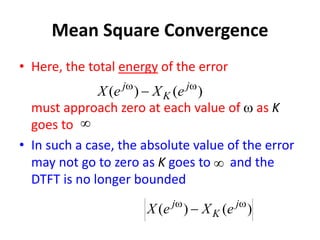
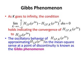
22. Mean Square Convergence
• To represent a finite energy sequence that is not
absolutely summable by a DTFT, it is necessary to
consider a mean-square convergence of
where
)
( w
j
e
X
0
)
(
)
(
lim
2

w
 



w
w


d
e
X
e
X j
K
j
K




w

w
K
K
n
n
j
j
K e
n
x
e
X ]
[
)
(

23. Mean Square Convergence
• Here, the total energy of the error
must approach zero at each value of w as K
goes to
• In such a case, the absolute value of the error
may not go to zero as K goes to and the
DTFT is no longer bounded


)
(
)
( w
w
 j
K
j
e
X
e
X
)
(
)
( w
w
 j
K
j
e
X
e
X

24. Example
• - Consider the DTFT
shown below





w

w
w

w


w
c
c
j
LP e
H
,
0
0
,
1
)
(
)
( w
j
LP e
H
c
w 
0
1

 c
w

w

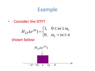
25. Example
• The inverse DTFT of is given by
• The energy of is given by
• is a finite-energy sequence, but
it is not absolutely summable
)
( w
j
LP e
H
]
[n
hLP
,
sin
2
1
n
n
jn
e
jn
e c
n
j
n
j c
c

w












w

w
w



w
w

w
d
e
n
h
c
c
n
j
LP
2
1
]
[




 n

w /
c
]
[n
hLP

26. Example
• As a result
does not uniformly converge to for all
values of w, but converges to in the
mean-square sense
)
( w
j
LP e
H
)
( w
j
LP e
H
 
w




w



w

K
K
n
n
j
c
K
K
n
n
j
LP e
n
n
e
n
h
sin
]
[

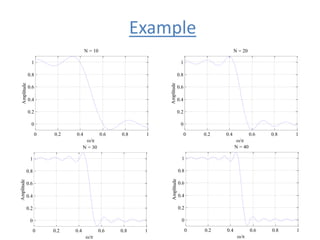
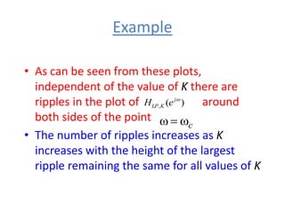
27. Example
• The mean-square convergence property of the
sequence can be further illustrated by
examining the plot of the function
for various values of K as shown next
 
w



w

w
K
K
n
n
j
c
j
K
LP e
n
n
e
H
sin
)
(
,
]
[n
hLP

28. Example
0 0.2 0.4 0.6 0.8 1
0
0.2
0.4
0.6
0.8
1
w/
Amplitude
N = 20
0 0.2 0.4 0.6 0.8 1
0
0.2
0.4
0.6
0.8
1
w/
Amplitude
N = 30
0 0.2 0.4 0.6 0.8 1
0
0.2
0.4
0.6
0.8
1
w/
Amplitude
N = 10
0 0.2 0.4 0.6 0.8 1
0
0.2
0.4
0.6
0.8
1
w/
Amplitude
N = 40

29. Example
• As can be seen from these plots,
independent of the value of K there are
ripples in the plot of around
both sides of the point
• The number of ripples increases as K
increases with the height of the largest
ripple remaining the same for all values of K
)
(
,
w
j
K
LP e
H
c
w

w

30. Gibbs Phenomenon
• As K goes to infinity, the condition
holds indicating the convergence of
to
• The oscillatory behavior of
approximating in the mean-square
sense at a point of discontinuity is known as
the Gibbs phenomenon
)
(
,
w
j
K
LP e
H
)
( w
j
LP e
H
0
)
(
)
(
lim
2
, 
w
 



w
w


d
e
H
e
H j
K
LP
j
LP
K
)
(
,
w
j
K
LP e
H
)
( w
j
LP e
H

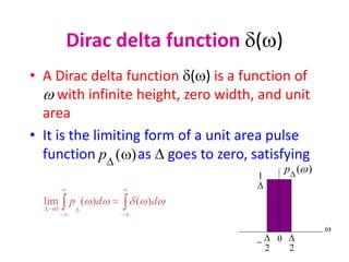
31. Dirac delta function d(w)
• The DTFT can also be defined for a certain
class of sequences which are neither
absolutely summable nor square summable
• Examples of such sequences are the unit step
sequence [n], the sinusoidal sequence
and the exponential sequence
• For this type of sequences, a DTFT
representation is possible using the Dirac delta
function d(w)
)
cos( 

w n
o
n
A

32. Dirac delta function d(w)
• A Dirac delta function d(w) is a function of
w with infinite height, zero width, and unit
area
• It is the limiting form of a unit area pulse
function as  goes to zero, satisfying
)
(w

p











 w
w
d
w
w d
d
p )
(
)
(
lim
0
w
2


2

0

1
)
(w

p

33. Example
• Example - Consider the complex exponential
sequence
• Its DTFT is given by
where is an impulse function of w and
n
j o
e
n
x w

]
[
 

w

w
d




w
k
o
j
k
e
X )
2
(
2
)
(
)
(w
d


w


 o

34. Example
• The function
is a periodic function of w with a period 2
and is called a periodic impulse train
• To verify that given above is indeed
the DTFT of we compute the
inverse DTFT of
 

w

w
d




w
k
o
j
k
e
X )
2
(
2
)
(
)
( w
j
e
X
n
j o
e
n
x w

]
[
)
( w
j
e
X

35. Example
• Thus
where we have used the sampling property of
the impulse function )
(w
d
  w


w

w
d








w
k
n
j
o d
e
k
n
x )
2
(
2
2
1
]
[
n
j
n
j
o
o
e
d
e w



w

w
 w

w
d
 )
(

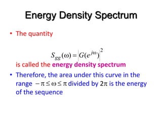
36. Energy Density Spectrum
• The total energy of a finite-energy sequence
g[n] is given by
• From Parseval’s relation given above we
observe that





n
g n
g
2
]
[
E
 w







w



d
e
G
n
g j
n
g
2
2
2
1
)
(
]
[
E

37. Energy Density Spectrum
• The quantity
is called the energy density spectrum
• Therefore, the area under this curve in the
range divided by 2 is the energy
of the sequence


w



2
)
(
)
( w

w j
gg e
G
S

38. Example
• - Compute the energy of the sequence
• Here
where






w
 n
n
n
n
h c
LP ,
sin
]
[
 w






w



d
e
H
n
h j
LP
n
LP
2
2
)
(
2
1
]
[





w

w
w

w


w
c
c
j
LP e
H
,
0
0
,
1
)
(

39. Energy Density Spectrum
• Therefore
• Hence, is a finite-energy sequence



w

 w



w
w




c
n
LP
c
c
d
n
h
2
1
]
[
2
]
[n
hLP