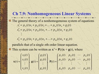
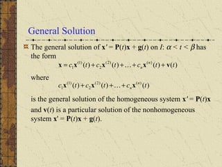
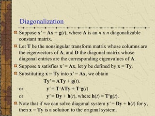
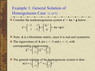
1) Nonhomogeneous linear systems generalize the theory of single nth order linear equations. They can be written in the form x' = P(t)x + g(t).
2) The general solution is the sum of the general solution to the homogeneous system x' = P(t)x and a particular solution to the nonhomogeneous system.
3) If the matrix P is constant and diagonalizable, the system can be transformed to uncoupled equations y' = Dy + h(t) via diagonalization, whose solutions give the solution to the original system.
Differential Equations Lecture: Non-Homogeneous Linear Differential Equationsbullardcr
A lecture I presented in Differential Equations, Spring 2006. This was supplemented with a hands-on solution to a random problem with variables designated by students in the class.
Differential Equations Lecture: Non-Homogeneous Linear Differential Equationsbullardcr
A lecture I presented in Differential Equations, Spring 2006. This was supplemented with a hands-on solution to a random problem with variables designated by students in the class.
This presentation gives the basic idea about the methods of solving ODEs
The methods like variation of parameters, undetermined coefficient method, 1/f(D) method, Particular integral and complimentary functions of an ODE
Numerical Solution of Nth - Order Fuzzy Initial Value Problems by Fourth Orde...IOSR Journals
In this paper, a numerical method for Nth - order fuzzy initial value problems (FIVP) based on
Seikkala derivative of fuzzy process is studied. The fourth order Runge-Kutta method based on Centroidal Mean
(RKCeM4) is used to find the numerical solution and the convergence and stability of the method is proved. This
method is illustrated by solving second and third order FIVPs. The results show that the proposed method suits
well to find the numerical solution of Nth – order FIVPs.
MAT210/DiffEq/Runge-Kutta 2nd Order 2013-14John Ham
Numerical methods lecture slides on the Runge-Kutta method for solving 1st order ODEs.
Some parts of this presentation are based on resources at http://nm.MathForCollege.com, primarily http://mathforcollege.com/nm/topics/runge_kutta_2nd_method.html
A set of notes prepared for an introductory machine learning course, assuming very limited linear algebra background, because all linear algebra operations are fully written out. These notes go into thorough derivations of the generalized linear regression formulation, demonstrating how to write it out in matrix form.
Continuous Time Convolution1. Solve the following for y(t.docxmaxinesmith73660
Continuous Time Convolution:
1. Solve the following for y(t)=x(t)*h(t)
x(t) = u(t)-u(t-4); h(t) = r(t)
2. Convolve the following:
3. Find the response of a system to an input of x(t)=2u(t-10) if h(t)=sin(2t)u(t).
4. A linear time invariant system has the following impulse response:
Use convolution to find the response y(t) to the following input:
Sketch y(t) for the case when a = 1.
h t e u tat( ) ( )= −2
x t u t u t( ) ( ) ( )= − − 4
5. Determine y(t) = x(t)*h(t) where x(t0 = u(t) and
6. Compute x(t)*v(t)
1
2
2 t
h(t)
1. a)
dy
dt
y t x t+ =6 4( ) ( )
This is an ordinary differential equation with constant coefficients, therefore, it is linear and time-
invariant. It contains memory and it is causal.
b)
dy
dt
ty t x t+ =4 2( ) ( )
This is an ordinary differential equation. The coefficients of 4t and 2 do not depend on y or x, so the
system is linear. However, the coefficient 4t is not constant, so it is time-varying. The system is also
causal and has memory
c)
This is a difference equation with constant coefficients; therefore, it is linear and time-invariant. It is
noncausal since the output depends on future values of x. Specifically, let x[n] = u[n], then y[-1] = 1.
d) y(t) = sin(x(t))
check linearity:
y t x t1 1( ) sin( ( ))=
y t x t2 2( ) sin( ( ))=
Solution
to an input of a x t a x t1 1 2 2( ) ( )+ is sin( ( ) ( ))a x t a x t1 1 2 2+ .
This is not equal to a y t a y t1 1 2 2( ) ( )+ .
As a counter example, consider x t1( ) = π and x t2 2( ) /= π , a a1 2 1= =
the system is causal since the output does not depend on future values of time, and it is memoryless
the system is time-invariant
e)
dy
dt
y t x t+ =2 ( ) ( )
The coefficient of y means that this is nonlinear; however, it does not depend explicitly on t, so it is time-
invariant. It is causal and has memory.
f) y n y n x n x n[ ] [ ] [ ] [ ]+ + = + −1 4 3 1
Rewrite the equation as y n y n x n x n[ ] [ ] [ ] [ ]+ − = − −4 1 3 1 by decreasing the index.
This is a difference equation with constant coefficients, so it is linear and time-invariant. The output does
not depend on future values of the input, so it is causal. It has memory.
y n y n x n[ ] [ ] [ ]+ − = +2 1 1
h) y n x n[ ] [ ]= 2
has memory since the output relies on values of the input at other the the current index n,
causal? Let x[n] = u[n-2], so x[1] = 0. Then y[1] = x[2] = 1, so not causal.
linear? Let y1 [n] = x1[2n] and y2 [n] = x2[2n]. The response to an input of x[n] = ax1[n]+bx2[n] is
y[n] = ax1[2n]+bx2[2n], which is ay1[2n]+by2[2n], so this is linear
time-invariant: Let y1[n] represent the response to an input of x[n-N], so y1[n] = x[2(n-N)]. This is also
equal to y[n-N], so the system is time-invariant.
i) y n nx n[ ] [ ]= 2
This is similar to part h), except for the n coefficient. Similar to above, it is noncausal, has memory and is
linear. Check time-invariance:
Let y1[n] represent the response to an input of x[n-N], so y1[n] =.
On the Application of the Fixed Point Theory to the Solution of Systems of Li...BRNSS Publication Hub
In this study, I worked on how to solve the biological and physical problems using systems of linear differential equations. A differential equation is an equation involving an unknown function and one or more of its derivatives. In this work, we consider systems of differential equations and their underlying theories illustrated with some solved examples. Finally, two applications, one to cell biology and the other to physical problems, were considered precisely.
Contemporary communication systems 1st edition mesiya solutions manualto2001
Contemporary Communication Systems 1st Edition Mesiya Solutions Manual
Download:https://goo.gl/DmVRQ4
contemporary communication systems mesiya pdf download
contemporary communication systems mesiya download
contemporary communication systems pdf
contemporary communication systems mesiya solutions
1. Ch 7.9: Nonhomogeneous Linear Systems
The general theory of a nonhomogeneous system of equations
parallels that of a single nth order linear equation.
This system can be written as x' = P(t)x + g(t), where
)()()()(
)()()()(
)()()()(
2211
222221212
112121111
tgxtpxtpxtpx
tgxtpxtpxtpx
tgxtpxtpxtpx
nnnnnnn
nn
nn
++++=′
++++=′
++++=′
=
=
=
)()()(
)()()(
)()()(
)(,
)(
)(
)(
)(,
)(
)(
)(
)(
21
22221
11211
2
1
2
1
tptptp
tptptp
tptptp
t
tg
tg
tg
t
tx
tx
tx
t
nnnn
n
n
nn
Pgx
2. General Solution
The general solution of x' = P(t)x + g(t) on I: α < t < β has
the form
where
is the general solution of the homogeneous system x' = P(t)x
and v(t) is a particular solution of the nonhomogeneous
system x' = P(t)x + g(t).
)()()()( )()2(
2
)1(
1 ttctctc n
n vxxxx ++++=
)()()( )()2(
2
)1(
1 tctctc n
nxxx +++
3. Diagonalization
Suppose x' = Ax + g(t), where A is an n x n diagonalizable
constant matrix.
Let T be the nonsingular transform matrix whose columns are
the eigenvectors of A, and D the diagonal matrix whose
diagonal entries are the corresponding eigenvalues of A.
Suppose x satisfies x' = Ax, let y be defined by x = Ty.
Substituting x = Ty into x' = Ax, we obtain
Ty' = ATy + g(t).
or y' = T-1
ATy + T-1
g(t)
or y' = Dy + h(t), where h(t) = T-1
g(t).
Note that if we can solve diagonal system y' = Dy + h(t) for y,
then x = Ty is a solution to the original system.
4. Solving Diagonal System
Now y' = Dy + h(t) is a diagonal system of the form
where r1,…, rn are the eigenvalues of A.
Thus y' = Dy + h(t) is an uncoupled system of n linear first
order equations in the unknowns yk(t), which can be isolated
and solved separately, using methods of Section 2.1:
+
=
′
′
′
⇔
++++=′
++++=′
++++=′
nnnnnnn
n
n
h
h
h
y
y
y
r
r
r
y
y
y
thyryyy
thyyryy
thyyyry
2
1
2
1
2
1
2
1
121
22212
12111
00
00
00
)(00
)(00
)(00
nkthyry kkk ,,1),(1 =+=′
nkecdssheey
t
t
tr
kk
srtr
k
kkk
,,1,)(
0
=+= ∫
−
5. Solving Original System
The solution y to y' = Dy + h(t) has components
For this solution vector y, the solution to the original system
x' = Ax + g(t) is then x = Ty.
Recall that T is the nonsingular transform matrix whose
columns are the eigenvectors of A.
Thus, when multiplied by T, the second term on right side of yk
produces general solution of homogeneous equation, while the
integral term of yk produces a particular solution of
nonhomogeneous system.
nkecdssheey
t
t
tr
kk
srtr
k
kkk
,,1,)(
0
=+= ∫
−
6. Example 1: General Solution of
Homogeneous Case (1 of 5)
Consider the nonhomogeneous system x' = Ax + g below.
Note: A is a Hermitian matrix, since it is real and symmetric.
The eigenvalues of A are r1 = -3 and r2 = -1, with
corresponding eigenvectors
The general solution of the homogeneous system is then
)(
3
2
21
12
t
t
e t
gAxxx +=
+
−
−
=′
−
=
−
=
1
1
,
1
1 )2()1(
ξξ
tt
ecect −−
+
−
=
1
1
1
1
)( 2
3
1x
7. Example 1: Transformation Matrix (2 of 5)
Consider next the transformation matrix T of eigenvectors.
Using a Section 7.7 comment, and A Hermitian, we have
T-1
= T*
= TT
, provided we normalize ξ(1)
and ξ(2)
so that (ξ(1)
,
ξ(1)
) = 1 and (ξ(2)
, ξ(2)
) = 1. Thus normalize as follows:
Then for this choice of eigenvectors,
=
+
=
−
=
−−−+
=
1
1
2
1
1
1
)1)(1()1)(1(
1
,
1
1
2
1
1
1
)1)(1()1)(1(
1
)2(
)1(
ξ
ξ
−
=
−
= −
11
11
2
1
,
11
11
2
1 1
TT
8. Example 1:
Diagonal System and its Solution (3 of 5)
Under the transformation x = Ty, we obtain the diagonal
system y' = Dy + T-1
g(t):
Then, using methods of Section 2.1,
+
−
+
−
−
=
−
+
−
−
=
′
′
−
−
−
te
te
y
y
t
e
y
y
y
y
t
t
t
32
32
2
13
3
2
11
11
2
1
10
03
2
1
2
1
2
1
( ) ttt
ttt
ectteyteyy
ec
t
eyteyy
−−−
−−−
+−+=⇒+=+′
+
−−=⇒−=+′
2222
3
1111
1
2
3
2
2
3
2
9
1
32
3
2
2
2
3
23
9. Example 1:
Transform Back to Original System (4 of 5)
We next use the transformation x = Ty to obtain the
solution to the original system x' = Ax + g(t):
( )
2
,
2
,
3
5
2
2
1
3
4
2
1
1
2
3
6
1
22
1
11
11
11
11
2
1
2
2
1
1
2
3
1
2
3
1
2
3
1
2
1
2
1
c
k
c
k
tetekek
tetekek
ektte
ek
t
e
y
y
x
x
ttt
ttt
tt
tt
==
+−+
−+−
+−+
++
=
+−+
+
−−
−
=
−
=
−−−
−−−
−−
−−
10. Example 1:
Solution of Original System (5 of 5)
Simplifying further, the solution x can be written as
Note that the first two terms on right side form the general
solution to homogeneous system, while the remaining terms
are a particular solution to nonhomogeneous system.
−
+
+
−
+
+
−
=
+−+
−+−
+−+
++
=
−−−−
−−−
−−−
5
4
3
1
2
1
1
1
1
1
2
1
1
1
1
1
3
5
2
2
1
3
4
2
1
2
3
1
2
3
1
2
3
1
2
1
tteeekek
tetekek
tetekek
x
x
tttt
ttt
ttt
11. Nondiagonal Case
If A cannot be diagonalized, (repeated eigenvalues and a
shortage of eigenvectors), then it can be transformed to its
Jordan form J, which is nearly diagonal.
In this case the differential equations are not totally
uncoupled, because some rows of J have two nonzero
entries: an eigenvalue in diagonal position, and a 1 in
adjacent position to the right of diagonal position.
However, the equations for y1,…, yn can still be solved
consecutively, starting with yn. Then the solution x to
original system can be found using x = Ty.
12. Undetermined Coefficients
A second way of solving x' = P(t)x + g(t) is the method of
undetermined coefficients. Assume P is a constant matrix,
and that the components of g are polynomial, exponential or
sinusoidal functions, or sums or products of these.
The procedure for choosing the form of solution is usually
directly analogous to that given in Section 3.6.
The main difference arises when g(t) has the form ueλt
,
where λ is a simple eigenvalue of P. In this case, g(t)
matches solution form of homogeneous system x' = P(t)x,
and as a result, it is necessary to take nonhomogeneous
solution to be of the form ateλt
+ beλt
. This form differs from
the Section 3.6 analog, ateλt
.
13. Example 2: Undetermined Coefficients (1 of 5)
Consider again the nonhomogeneous system x' = Ax + g:
Assume a particular solution of the form
where the vector coefficents a, b, c, d are to be determined.
Since r = -1 is an eigenvalue of A, it is necessary to include
both ate-t
and be-t
, as mentioned on the previous slide.
te
t
e t
t
+
+
−
−
=
+
−
−
=′ −
−
3
0
0
2
21
12
3
2
21
12
xxx
dcbav +++= −−
tetet tt
)(
14. Example 2:
Matrix Equations for Coefficients (2 of 5)
Substituting
in for x in our nonhomogeneous system x' = Ax + g,
we obtain
Equating coefficients, we conclude that
,
3
0
0
2
21
12
te t
+
+
−
−
=′ −
xx
dcbav +++= −−
tetet tt
)(
cAdAcbaAbaAa =
−=
−−=−= ,
3
0
,
0
2
,
( ) teteteete ttttt
+
++++=+−+− −−−−−
3
0
0
2
AdAcAbAacbaa
15. Example 2:
Solving Matrix Equation for a (3 of 5)
Our matrix equations for the coefficients are:
From the first equation, we see that a is an eigenvector of A
corresponding to eigenvalue r = -1, and hence has the form
We will see on the next slide that α = 1, and hence
cAdAcbaAbaAa =
−=
−−=−= ,
3
0
,
0
2
,
=
α
α
a
=
1
1
a
16. Example 2:
Solving Matrix Equation for b (4 of 5)
Our matrix equations for the coefficients are:
Substituting aT
= (α,α) into second equation,
Thus α = 1, and solving for b, we obtain
cAdAcbaAbaAa =
−=
−−=−= ,
3
0
,
0
2
,
−
=
−
⇔
−
=
−
−
⇔
−
=
+
−
−
⇔
−
−
=
100
112
11
11
2
10
01
21
122
2
1
2
1
2
1
2
1
α
α
α
α
α
α
α
α
b
b
b
b
b
b
b
b
Ab
−
=→=→
−
=
1
0
0choose
1
0
1
1
bb kk
17. Example 2: Particular Solution (5 of 5)
Our matrix equations for the coefficients are:
Solving third equation for c, and then fourth equation for d,
it is straightforward to obtain cT
= (1, 2), dT
= (-4/3, -5/3).
Thus our particular solution of x' = Ax + g is
Comparing this to the result obtained in Example 1, we see
that both particular solutions would be the same if we had
chosen k = ½ for b on previous slide, instead of k = 0.
cAdAcbaAbaAa =
−=
−−=−= ,
3
0
,
0
2
,
−
+
−
= −−
5
4
3
1
2
1
1
0
1
1
)( tetet tt
v
18. Variation of Parameters: Preliminaries
A more general way of solving x' = P(t)x + g(t) is the
method of variation of parameters.
Assume P(t) and g(t) are continuous on α < t < β, and let
Ψ(t) be a fundamental matrix for the homogeneous system.
Recall that the columns of Ψ are linearly independent
solutions of x' = P(t)x, and hence Ψ(t) is invertible on the
interval α < t < β, and also Ψ'(t) = P(t)Ψ(t).
Next, recall that the solution of the homogeneous system
can be expressed as x = Ψ(t)c.
Analogous to Section 3.7, assume the particular solution of
the nonhomogeneous system has the form x = Ψ(t)u(t),
where u(t) is a vector to be found.
19. Variation of Parameters: Solution
We assume a particular solution of the form x = Ψ(t)u(t).
Substituting this into x' = P(t)x + g(t), we obtain
Ψ'(t)u(t) + Ψ(t)u'(t) = P(t)Ψ(t)u(t) + g(t)
Since Ψ'(t) = P(t)Ψ(t), the above equation simplifies to
u'(t) = Ψ-1
(t)g(t)
Thus
where the vector c is an arbitrary constant of integration.
The general solution to x' = P(t)x + g(t) is therefore
cΨu += ∫
−
dttgtt )()()( 1
( ) arbitrary,,)()()()( 1
1
1
βα∈+= ∫
−
tdssstt
t
t
gΨΨcΨx
20. Variation of Parameters: Initial Value Problem
For an initial value problem
x' = P(t)x + g(t), x(t0) = x(0)
,
the general solution to x' = P(t)x + g(t) is
Alternatively, recall that the fundamental matrix Φ(t)
satisfies Φ(t0) = I, and hence the general solution is
In practice, it may be easier to row reduce matrices and
solve necessary equations than to compute Ψ-1
(t) and
substitute into equations. See next example.
∫
−−
+=
t
t
dsssttt
0
)()()()()( 1)0(
0
1
gΨΨxΨΨx
∫
−
+=
t
t
dssstt
0
)()()()( 1)0(
gΨΦxΦx
21. Example 3: Variation of Parameters (1 of 3)
Consider again the nonhomogeneous system x' = Ax + g:
We have previously found general solution to homogeneous
case, with corresponding fundamental matrix:
Using variation of parameters method, our solution is given
by x = Ψ(t)u(t), where u(t) satisfies Ψ(t)u'(t) = g(t), or
te
t
e t
t
+
+
−
−
=
+
−
−
=′ −
−
3
0
0
2
21
12
3
2
21
12
xxx
−
= −−
−−
tt
tt
ee
ee
t 3
3
)(Ψ
=
′
′
−
−
−−
−−
t
e
u
u
ee
ee t
tt
tt
3
2
2
1
3
3
22. Example 3: Solving for u(t) (2 of 3)
Solving Ψ(t)u'(t) = g(t) by row reduction,
It follows that
2/31
2/3
2/3110
2/301
2/30
2/30
2/30
2
3220
2
3
2
2
32
1
32
33
3
3
3
t
tt
t
tt
tt
tt
tt
ttt
tt
ttt
tt
ttt
teu
teeu
te
tee
tee
tee
tee
eee
tee
eee
tee
eee
+=′
−=′
→
+
−
→
+
−
→
+
→
+
→
−
−−
−−
−−
−−−
−−
−−−
−−
−−−
+−+
++−
=
=
2
1
332
2
1
2/32/3
6/2/2/
)(
cetet
cetee
u
u
t tt
ttt
u
23. Example 3: Solving for x(t) (3 of 3)
Now x(t) = Ψ(t)u(t), and hence we multiply
to obtain, after collecting terms and simplifying,
Note that this is the same solution as in Example 1.
+−+
++−
−
= −−
−−
2
1
332
3
3
2/32/3
6/2/2/
cetet
cetee
ee
ee
tt
ttt
tt
tt
x
−
+
−
+
+
+
−
= −−−−
5
4
3
1
2
1
1
1
2
1
1
1
1
1
1
1
2
3
1 teteecec tttt
x
24. Laplace Transforms
The Laplace transform can be used to solve systems of
equations. Here, the transform of a vector is the vector of
component transforms, denoted by X(s):
Then by extending Theorem 6.2.1, we obtain
{ }
{ }
{ }
)(
)(
)(
)(
)(
)(
2
1
2
1
s
txL
txL
tx
tx
LtL Xx =
=
=
{ } )0()()( xXx −=′ sstL
25. Example 4: Laplace Transform (1 of 5)
Consider again the nonhomogeneous system x' = Ax + g:
Taking the Laplace transform of each term, we obtain
where G(s) is the transform of g(t), and is given by
+
−
−
=′
−
t
e t
3
2
21
12
xx
( )
+
= 2
3
12
)(
s
s
sG
)()()0()( ssss GAXxX +=−
26. Example 4: Transfer Matrix (2 of 5)
Our transformed equation is
If we take x(0) = 0, then the above equation becomes
or
Solving for X(s), we obtain
The matrix (sI – A)-1
is called the transfer matrix.
)()()0()( ssss GAXxX +=−
)()()( ssss GAXX +=
( ) )()(
1
sss GAIX
−
−=
( ) )()( sss GXAI =−
27. Example 4: Finding Transfer Matrix (3 of 5)
Then
Solving for (sI – A)-1
, we obtain
( )
+−
−+
=−⇒
−
−
=
21
12
21
12
s
s
s AIA
( )
+
+
++
=−
−
21
12
)3)(1(
11
s
s
ss
s AI
28. Example 4: Transfer Matrix (4 of 5)
Next, X(s) = (sI – A)-1
G(s), and hence
or
+
+
+
++
= 2
3
)1(2
21
12
)3)(1(
1
)(
s
s
s
s
ss
sX
( )
( ) ( )
( ) ( )
++
+
+
++
++
+
++
+
=
)3(1
)2(3
)3(1
2
)3(1
3
)3(1
22
)(
22
22
sss
s
ss
sssss
s
sX
29. Example 4: Transfer Matrix (5 of 5)
Thus
To solve for x(t) = L-1
{X(s)}, use partial fraction expansions
of both components of X(s), and then Table 6.2.1 to obtain:
Since we assumed x(0) = 0, this solution differs slightly
from the previous particular solutions.
( )
( ) ( )
( ) ( )
++
+
+
++
++
+
++
+
=
)3(1
)2(3
)3(1
2
)3(1
3
)3(1
22
)(
22
22
sss
s
ss
sssss
s
sX
−
+
+
+
−
−= −−−
5
4
3
1
2
1
1
1
1
2
1
1
3
2 3
tteee ttt
x
30. Summary (1 of 2)
The method of undetermined coefficients requires no
integration but is limited in scope and may involve several
sets of algebraic equations.
Diagonalization requires finding inverse of transformation
matrix and solving uncoupled first order linear equations.
When coefficient matrix is Hermitian, the inverse of
transformation matrix can be found without calculation,
which is very helpful for large systems.
The Laplace transform method involves matrix inversion,
matrix multiplication, and inverse transforms. This method
is particularly useful for problems with discontinuous or
impulsive forcing functions.
31. Summary (2 of 2)
Variation of parameters is the most general method, but it
involves solving linear algebraic equations with variable
coefficients, integration, and matrix multiplication, and
hence may be the most computationally complicated
method.
For many small systems with constant coefficients, all of
these methods work well, and there may be little reason to
select one over another.