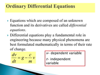
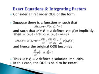
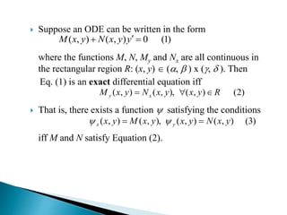
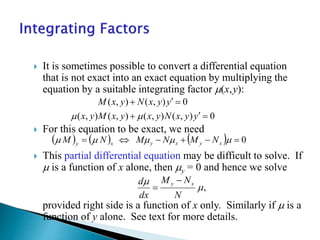
- Differential equations relate an unknown function and its derivatives, and are classified as ordinary (ODE) or partial (PDE) depending on the number of independent variables. Higher order equations can be reduced to systems of first order equations. - Exact differential equations can be written as the total differential of a function, while non-exact equations may require an integrating factor to convert them to exact form. 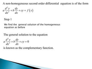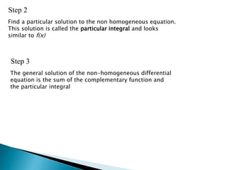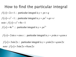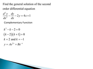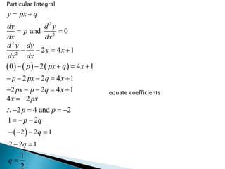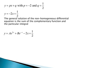- The general solution to a non-homogeneous second order differential equation is the sum of the complementary function (solution to the homogeneous equation) and a particular integral similar to the non-homogeneous term.

2.  Equations which are composed of an unknown
function and its derivatives are called differential
equations.
 Differential equations play a fundamental role in
engineering because many physical phenomena are
best formulated mathematically in terms of their rate
of change.
v- dependent variable
t- independent
variable
v
m
c
g
dt
dv


3.  When a function involves one dependent variable, the
equation is called an ordinary differential equation
(or ODE). A partial differential equation (or PDE)
involves two or more independent variables.
 Differential equations are also classified as to their
order.
 A first order equation includes a first derivative as its
highest derivative.
 A second order equation includes a second derivative.
 Higher order equations can be reduced to a system of
first order equations, by redefining a variable.

4.  Consider a first order ODE of the form
 Suppose there is a function  such that
and such that (x,y) = c defines y = (x) implicitly.
Then
and hence the original ODE becomes
 Thus (x,y) = c defines a solution implicitly.
 In this case, the ODE is said to be exact.
0),(),(  yyxNyxM
),(),(),,(),( yxNyxyxMyx yx  
 )(,),(),( xx
dx
d
dx
dy
yx
yyxNyxM 








  0)(, xx
dx
d


5.  Suppose an ODE can be written in the form
where the functions M, N, My and Nx are all continuous in
the rectangular region R: (x, y)  (,  ) x (,  ). Then
Eq. (1) is an exact differential equation iff
 That is, there exists a function  satisfying the conditions
iff M and N satisfy Equation (2).
)1(0),(),(  yyxNyxM
)2(),(),,(),( RyxyxNyxM xy 
)3(),(),(),,(),( yxNyxyxMyx yx  

6.  It is sometimes possible to convert a differential equation
that is not exact into an exact equation by multiplying the
equation by a suitable integrating factor (x,y):
 For this equation to be exact, we need
 This partial differential equation may be difficult to solve. If
 is a function of x alone, then y = 0 and hence we solve
provided right side is a function of x only. Similarly if  is a
function of y alone. See text for more details.
0),(),(),(),(
0),(),(


yyxNyxyxMyx
yyxNyxM

      0  xyxyxy NMNMNM
,

N
NM
dx
d xy 


8.  
2
2
A non-homogeneous second order differential equation is of the form
d y dy
a b cy f x
dx dx
  
We find the general solution of the homogeneous
equation as before
2
2
The general solution to the equation
0
is known as the complementary function.
d y dy
a b cy
dx dx
  
Step 1

9. Step 2
Find a particular solution to the non homogeneous equation.
This solution is called the particular integral and looks
similar to f(x)
Step 3
The general solution of the non-homogeneous differential
equation is the sum of the complementary function and
the particular integral

11.   2 1 particular integral isf x x y px q    
 
 
2 2
2
1 particular integral is
: 0 1
f x x y px qx r
note f x x x
     
  
  2 2
4 particular integral isx x
f x e y pe  
  2sin cos particular integral is sin cosf x x x y p x q x    
 
 
3sin 2 particular integral is sin 2 cos2
: 3sin 2 0cos2
f x x y p x q x
note f x x x
   
 

12. 2
2
Find the general solution of the second
order differential equation
2 4 1
d y dy
y x
dx dx
   
  
2
2
2 0
2 1 0
2 and 1
x x
k k
k k
k k
y Ae Be
  
  
  
 
Complementary Function

13. Particular Integral
2
2
and 0
y px q
dy d y
p
dx dx
 
 
     
2
2
2 4 1
0 2 4 1
2 2 4 1
2 2 4 1
d y dy
y x
dx dx
p px q x
p px q x
px p q x
   
    
    
     equate coefficients
4 2
2 4 and 2
x px
p p
 
   
 
1 2
2 2 1
2 2 1
1
2
p q
q
q
q
  
   
 


14. The general solution of the non-homogeneous differential
equation is the sum of the complementary function and
the particular integral
2 1
2
2
x x
y Ae Be x
   
1
with 2 and
2
1
2
2
y px q p q
y x
    
  