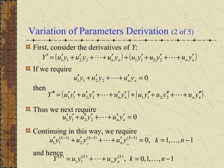
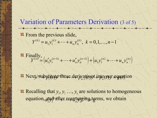
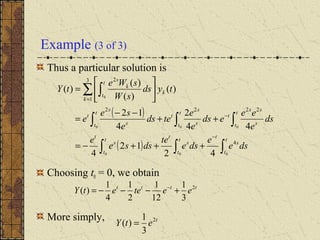
The variation of parameters method can be used to find particular solutions to nonhomogeneous linear differential equations. It involves: 1) Assuming the particular solution (Y) is a linear combination of the fundamental solutions to the homogeneous equation, with coefficients (u1, u2,...un) that are functions to be determined. 2) Deriving n equations for the n unknown functions by substituting Y and its derivatives into the original differential equation. 3) Solving the n equations using Cramer's rule to obtain expressions for the n functions, which can then be integrated to give the particular solution Y.

1. Ch 4.4: Variation of Parameters
The variation of parameters method can be used to find a
particular solution of the nonhomogeneous nth order linear
differential equation
provided g is continuous.
As with 2nd
order equations, begin by assuming y1, y2 …, yn are
fundamental solutions to homogeneous equation.
Next, assume the particular solution Y has the form
where u1, u2,… un are functions to be solved for.
In order to find these n functions, we need n equations.
[ ] ),()()()( 1
)1(
1
)(
tgytpytpytpyyL nn
nn
=+′+++= −
−

)()()()()()()( 2211 tytutytutytutY nn+++= 

2. Variation of Parameters Derivation (2 of 5)
First, consider the derivatives of Y:
If we require
then
Thus we next require
Continuing in this way, we require
and hence
( ) ( )nnnn yuyuyuyuyuyuY ′++′+′+′++′+′=′  22112211
02211 =′++′+′ nn yuyuyu 
( ) ( )nnnn yuyuyuyuyuyuY ′′++′′+′′+′′++′′+′′=′′  22112211
02211 =′′++′′+′′ nn yuyuyu 
1,,1,0)1()1(
2
)1(
11 2
−==′++′+′ −−−
nkyuyuyu k
n
kk
n

1,,1,0,)()(
11
)(
−=++= nkyuyuY k
nn
kk


3. Variation of Parameters Derivation (3 of 5)
From the previous slide,
Finally,
Next, substitute these derivatives into our equation
Recalling that y1, y2 …, yn are solutions to homogeneous
equation, and after rearranging terms, we obtain
( ) ( ))()(
11
)1()1(
11
)( n
nn
nn
nn
nn
yuyuyuyuY +++′++′= −−

1,,1,0,)()(
11
)(
−=++= nkyuyuY k
nn
kk

gyuyu n
nn
n
=′++′ −− )1()1(
11 
)()()()( 1
)1(
1
)(
tgytpytpytpy nn
nn
=+′+++ −
−


4. Variation of Parameters Derivation (4 of 5)
The n equations needed in order to find the n functions
u1, u2,… un are
Using Cramer’s Rule, for each k = 1, …, n,
and Wk is determinant obtained by replacing kth column of
W with (0, 0, …, 1).
gyuyu
yuyu
yuyu
n
nn
n
nn
n
=′++′
=′′++′′
=′++′
−− )1()1(
11
11
111
0
0




))(,,()(where,
)(
)()(
)( 1 tyyWtW
tW
tWtg
tu n
k
k ==′

5. Variation of Parameters Derivation (5 of 5)
From the previous slide,
Integrate to obtain u1, u2,… un:
Thus, a particular solution Y is given by
where t0 is arbitrary.
nk
tW
tWtg
tu k
k ,,1,
)(
)()(
)( ==′
nkds
sW
sWsg
tu
t
t
k
k ,,1,
)(
)()(
)(
0
== ∫
∑ ∫=






=
n
k
k
t
t
k
tyds
sW
sWsg
tY
1
)(
)(
)()(
)(
0

6. Example (1 of 3)
Consider the equation below, along with the given solutions
of corresponding homogeneous solutions y1, y2, y3:
Then a particular solution of this ODE is given by
It can be shown that
tttt
etytetyetyeyyyy −
====+′−′′−′′′ )(,)(,)(, 321
2
∑ ∫=






=
3
1
2
)(
)(
)(
)(
0
k
k
t
t
k
s
tyds
sW
sWe
tY
( )
( )
t
ttt
ttt
ttt
e
eete
eete
etee
tW 4
2
1)( =
+
−+=
−
−
−

7. Example (2 of 3)
Also,
( )
( )
( )
( )
t
tt
tt
tt
tt
tt
tt
tt
tt
tt
e
ete
ete
tee
tW
ee
ee
ee
tW
t
eet
eet
ete
tW
=
+
+=
=−=
−−=
+
−+=
−
−
−
−
−
−
12
01
0
)(
2
1
0
0
)(
12
21
10
0
)(
3
2
1

8. Example (3 of 3)
Thus a particular solution is
Choosing t0 = 0, we obtain
More simply,
( )
( ) ∫∫∫
∫∫∫
∑ ∫
−
−
=
+++−=
++
−−
=






=
t
t
s
t
t
t
s
t
t
t
s
t
t
t s
ss
t
t
t s
s
t
t
t s
s
t
k
k
t
t
k
s
dse
e
dse
te
dsse
e
ds
e
ee
eds
e
e
teds
e
se
e
tyds
sW
sWe
tY
000
000
0
4
2222
3
1
2
42
12
4
44
2
4
12
)(
)(
)(
)(
tttt
eeteetY 2
3
1
12
1
2
1
4
1
)( +−−−= −
t
etY 2
3
1
)( =