Downloaded 15 times

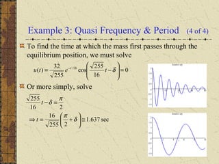
![Spring Model:
Spring Force Details
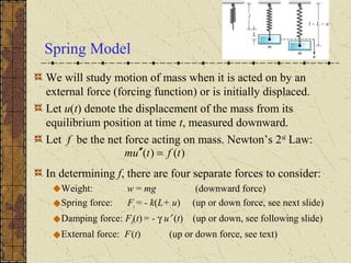
The spring force Fs acts to restore spring to natural position,
and is proportional to L + u. If L + u > 0, then spring is
extended and the spring force acts upward. In this case
If L + u < 0, then spring is compressed a distance of |L + u|,
and the spring force acts downward. In this case
In either case,
)( uLkFs +−=
( )[ ] ( )uLkuLkuLkFs +−=+−=+=
)( uLkFs +−=](https://image.slidesharecdn.com/ch038-150731094636-lva1-app6891/85/Ch03-8-4-320.jpg)
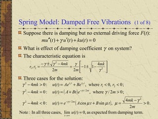
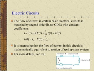
![Spring Model:
Differential Equation
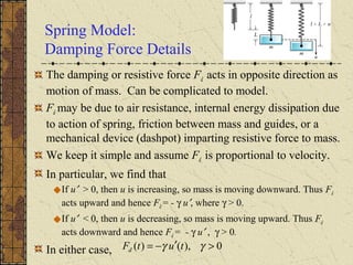
Taking into account these forces, Newton’s Law becomes:
Recalling that mg = kL, this equation reduces to
where the constants m, γ, and k are positive.
We can prescribe initial conditions also:
It follows from Theorem 3.2.1 that there is a unique solution
to this initial value problem. Physically, if mass is set in
motion with a given initial displacement and velocity, then
its position is uniquely determined at all future times.
[ ] )()()(
)()()()(
tFtutuLkmg
tFtFtFmgtum ds
+′−+−=
+++=′′
γ
)()()()( tFtkututum =+′+′′ γ
00 )0(,)0( vuuu =′=](https://image.slidesharecdn.com/ch038-150731094636-lva1-app6891/85/Ch03-8-6-320.jpg)
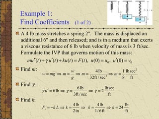
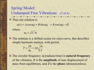
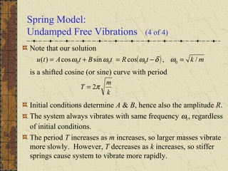
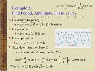
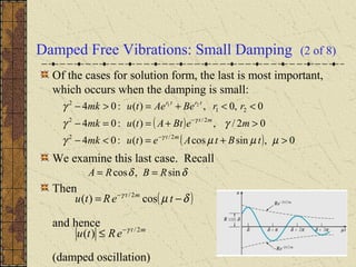
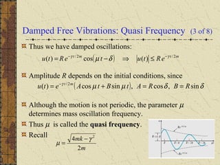
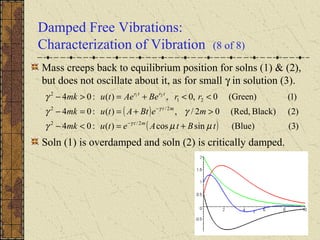
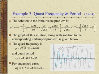
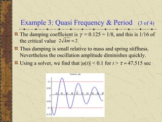

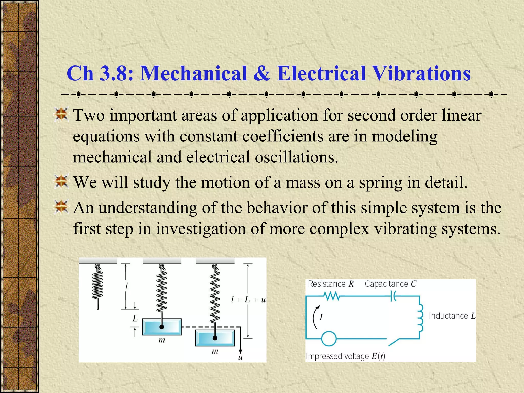
The motion of a mass attached to a spring can be modeled by a second order differential equation. For undamped free vibrations with no external force, the solution is a simple harmonic motion with natural frequency ω0 and period T. Small damping causes the motion to be damped oscillations with slightly reduced quasi-frequency μ and increased quasi-period Td. The ratio γ2/4km determines whether damping can be neglected - if small, damping has little effect on frequency and period.


