This document discusses fundamental solutions of linear homogeneous differential equations. It introduces the concept of a fundamental set of solutions - two solutions whose Wronskian is nonzero at some point. Any linear combination of a fundamental set with arbitrary constants forms the general solution. The principle of superposition and Wronskian determinant are used to show whether a given set of solutions spans all solutions. Examples demonstrate finding fundamental solutions and using them to solve initial value problems. Theorems establish existence and properties of fundamental solutions, including their role in solving initial value problems uniquely.

1. Ch 3.2: Fundamental Solutions of Linear
Homogeneous Equations
Let p, q be continuous functions on an interval I = (α, β),
which could be infinite. For any function y that is twice
differentiable on I, define the differential operator L by
Note that L[y] is a function on I, with output value
For example,
[ ] yqypyyL +′+′′=
[ ] )()()()()()( tytqtytptytyL +′+′′=
( )
[ ] )sin(2)cos()sin()(
2,0),sin()(,)(,)(
22
22
tettttyL
Ittyetqttp
t
t
++−=
==== π

2. Differential Operator Notation
In this section we will discuss the second order linear
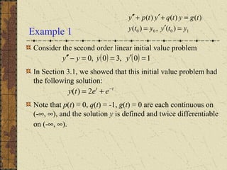
homogeneous equation L[y](t) = 0, along with initial
conditions as indicated below:
We would like to know if there are solutions to this initial
value problem, and if so, are they unique.
Also, we would like to know what can be said about the form
and structure of solutions that might be helpful in finding
solutions to particular problems.
These questions are addressed in the theorems of this section.
[ ]
1000 )(,)(
0)()(
ytyyty
ytqytpyyL
=′=
=+′+′′=

3. Theorem 3.2.1
Consider the initial value problem
where p, q, and g are continuous on an open interval I that
contains t0. Then there exists a unique solution y = φ(t) on I.
Note: While this theorem says that a solution to the initial
value problem above exists, it is often not possible to write
down a useful expression for the solution. This is a major
difference between first and second order linear equations.
0000 )(,)(
)()()(
ytyyty
tgytqytpy
′=′=
=+′+′′

4. Example 1
Consider the second order linear initial value problem
In Section 3.1, we showed that this initial value problem had
the following solution:
Note that p(t) = 0, q(t) = -1, g(t) = 0 are each continuous on
(-∞, ∞), and the solution y is defined and twice differentiable
on (-∞, ∞).
tt
eety −
+= 2)(
( ) ( ) 10,30,0 =′==−′′ yyyy
1000 )(,)(
)()()(
ytyyty
tgytqytpy
=′=
=+′+′′

5. Example 2
Consider the second order linear initial value problem
where p, q are continuous on an open interval I containing t0.
In light of the initial conditions, note that y = 0 is a solution
to this homogeneous initial value problem.
Since the hypotheses of Theorem 3.2.1 are satisfied, it
follows that y = 0 is the only solution of this problem.
( ) ( ) 00,00,0)()( =′==+′+′′ yyytqytpy

6. Example 3
Determine the longest interval on which the given initial
value problem is certain to have a unique twice
differentiable solution. Do not attempt to find the solution.
First put differential equation into standard form:
The longest interval containing the point t = 0 on which the
coefficient functions are continuous is (-1, ∞).
It follows from Theorem 3.2.1 that the longest interval on
which this initial value problem is certain to have a twice
differentiable solution is also (-1, ∞).
( ) ( ) ( ) 00,10,13)(cos1 =′==+′−′′+ yyyytyt
( ) ( ) 00,10,
1
1
1
3
1
cos
=′=
+
=
+
+′
+
−′′ yy
t
y
t
y
t
t
y

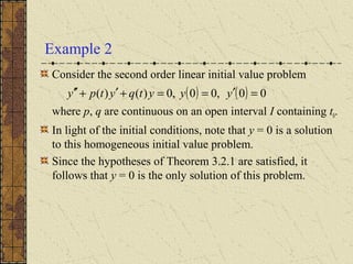
7. Theorem 3.2.2 (Principle of Superposition)
If y1and y2 are solutions to the equation
then the linear combination c1y1 + y2c2 is also a solution, for
all constants c1 and c2.
To prove this theorem, substitute c1y1 + y2c2 in for y in the
equation above, and use the fact that y1 and y2 are solutions.
Thus for any two solutions y1and y2, we can construct an
infinite family of solutions, each of the form y = c1y1 + c2 y2.
Can all solutions can be written this way, or do some
solutions have a different form altogether? To answer this
question, we use the Wronskian determinant.
0)()(][ =+′+′′= ytqytpyyL

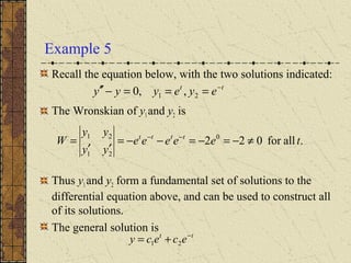
8. The Wronskian Determinant (1 of 3)
Suppose y1 and y2 are solutions to the equation
From Theorem 3.2.2, we know that y = c1y1 + c2y2 is a solution
to this equation.
Next, find coefficients such that y = c1y1 + c2y2 satisfies the
initial conditions
To do so, we need to solve the following equations:
0)()(][ =+′+′′= ytqytpyyL
0000 )(,)( ytyyty ′=′=
0022011
0022011
)()(
)()(
ytyctyc
ytyctyc
′=′+′
=+

9. The Wronskian Determinant (2 of 3)
Solving the equations, we obtain
In terms of determinants:
0022011
0022011
)()(
)()(
ytyctyc
ytyctyc
′=′+′
=+
)()()()(
)()(
)()()()(
)()(
02010201
010010
2
02010201
020020
1
tytytyty
tyytyy
c
tytytyty
tyytyy
c
′−′
′+′−
=
′−′
′−′
=
)()(
)()(
)(
)(
,
)()(
)()(
)(
)(
0201
0201
001
001
2
0201
0201
020
020
1
tyty
tyty
yty
yty
c
tyty
tyty
tyy
tyy
c
′′
′′
=
′′
′′
=

10. The Wronskian Determinant (3 of 3)
In order for these formulas to be valid, the determinant W in
the denominator cannot be zero:
W is called the Wronskian determinant, or more simply,
the Wronskian of the solutions y1and y2. We will sometimes
use the notation
)()()()(
)()(
)()(
02010201
0201
0201
tytytyty
tyty
tyty
W ′−′=
′′
=
W
yty
yty
c
W
tyy
tyy
c 001
001
2
020
020
1
)(
)(
,
)(
)(
′′
=
′′
=
( )( )021, tyyW

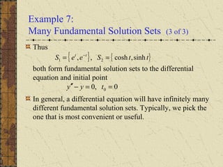
11. Theorem 3.2.3
Suppose y1and y2 are solutions to the equation
and that the Wronskian
is not zero at the point t0where the initial conditions
are assigned. Then there is a choice of constants c1, c2 for
which y = c1y1 + c2y2 is a solution to the differential equation
(1) and initial conditions (2).
)1(0)()(][ =+′+′′= ytqytpyyL
2121 yyyyW ′−′=
)2()(,)( 0000 ytyyty ′=′=

12. Example 4
Recall the following initial value problem and its solution:
Note that the two functions below are solutions to the
differential equation:
The Wronskian of y1and y2 is
Since W ≠ 0 for all t, linear combinations of y1and y2 can be
used to construct solutions of the IVP for any initial value t0.
tt
eyey −
== 21 ,
22 0
2121
21
21
−=−=−−=′−′=
′′
= −−
eeeeeyyyy
yy
yy
W tttt
( ) ( ) tt
eetyyyyy −
+=⇒=′==−′′ 2)(10,30,0
2211 ycycy +=

13. Theorem 3.2.4 (Fundamental Solutions)
Suppose y1and y2 are solutions to the equation
If there is a point t0 such that W(y1,y2)(t0) ≠ 0, then the family
of solutions y = c1y1 + c2y2 with arbitrary coefficients c1, c2
includes every solution to the differential equation.
The expression y = c1y1 + c2y2 is called the general solution
of the differential equation above, and in this case y1 and y2
are said to form a fundamental set of solutions to the
differential equation.
.0)()(][ =+′+′′= ytqytpyyL

14. Example 5
Recall the equation below, with the two solutions indicated:
The Wronskian of y1and y2 is
Thus y1 and y2 form a fundamental set of solutions to the
differential equation above, and can be used to construct all
of its solutions.
The general solution is
tt
eyeyyy −
===−′′ 21 ,,0
.allfor022 0
21
21
teeeee
yy
yy
W tttt
≠−=−=−−=
′′
= −−
tt
ececy −
+= 21

15. Example 6
Consider the general second order linear equation below,
with the two solutions indicated:
Suppose the functions below are solutions to this equation:
The Wronskian of y1and y2 is
Thus y1and y2 form a fundamental set of solutions to the
equation, and can be used to construct all of its solutions.
The general solution is
2121 ,, 21
rreyey trtr
≠==
( ) ( )
.allfor021
21
21
12
2121
21
terr
erer
ee
yy
yy
W trr
trtr
trtr
≠−==
′′
= +
0)()( =+′+′′ ytqytpy
trtr
ececy 21
21 +=

16. Example 7: Solutions (1 of 2)
Consider the following differential equation:
Show that the functions below are fundamental solutions:
To show this, first substitute y1 into the equation:
Thus y1 is a indeed a solution of the differential equation.
Similarly, y2 is also a solution:
1
2
2/1
1 , −
== tyty
0,032 2
>=−′+′′ tyytyt
01
2
3
2
1
2
3
4
2 2/12/1
2/12/3
2
=





−+−=−





+




 − −−
tt
t
t
t
t
( ) ( ) ( ) 0134322 11232
=−−=−−+ −−−−
tttttt

17. Example 7: Fundamental Solutions (2 of 2)
Recall that
To show that y1and y2 form a fundamental set of solutions,
we evaluate the Wronskian of y1and y2:
Since W ≠ 0 for t > 0, y1, y2 form a fundamental set of
solutions for the differential equation
3
2/32/32/3
22/1
12/1
21
21
2
3
2
3
2
1
2
1
t
ttt
tt
tt
yy
yy
W −=−=−−=
−
=
′′
= −−−
−−
−
1
2
2/1
1 , −
== tyty
0,032 2
>=−′+′′ tyytyt

18. Theorem 3.2.5: Existence of Fundamental Set
of Solutions
Consider the differential equation below, whose coefficients
p and q are continuous on some open interval I:
Let t0be a point in I, and y1 and y2 solutions of the equation
with y1 satisfying initial conditions
and y2 satisfying initial conditions
Then y1, y2 form a fundamental set of solutions to the given
differential equation.
0)()(][ =+′+′′= ytqytpyyL
0)(,1)( 0101 =′= tyty
1)(,0)( 0202 =′= tyty

19. Example 7: Theorem 3.2.5 (1 of 3)
Find the fundamental set specified by Theorem 3.2.5 for the
differential equation and initial point
We showed previously that
were fundamental solutions, since W(y1, y2)(t0) = -2 ≠ 0.
But these two solutions don’t satisfy the initial conditions
stated in Theorem 3.2.5, and thus they do not form the
fundamental set of solutions mentioned in that theorem.
Let y3and y4 be the fundamental solutions of Thm 3.2.5.
tt
eyey −
== 21 ,
0,0 0 ==−′′ tyy
1)0(,0)0(;0)0(,1)0( 4433 =′==′= yyyy

20. Example 7: General Solution (2 of 3)
Since y1 and y2 form a fundamental set of solutions,
Solving each equation, we obtain
The Wronskian of y3and y4 is
Thus y3, y4 forms the fundamental set of solutions indicated
in Theorem 3.2.5, with general solution in this case
1)0(,0)0(,
0)0(,1)0(,
44214
33213
=′=+=
=′=+=
−
−
yyededy
yyececy
tt
tt
)sinh(
2
1
2
1
)(),cosh(
2
1
2
1
)( 43 teetyteety tttt
=−==+= −−
01sinhcosh
coshsinh
sinhcosh 22
21
21
≠=−==
′′
= tt
tt
tt
yy
yy
W
)sinh()cosh()( 21 tktkty +=

21. Example 7:
Many Fundamental Solution Sets (3 of 3)
Thus
both form fundamental solution sets to the differential
equation and initial point
In general, a differential equation will have infinitely many
different fundamental solution sets. Typically, we pick the
one that is most convenient or useful.
{ } { }ttSeeS tt
sinh,cosh,, 21 == −
0,0 0 ==−′′ tyy

22. Summary
To find a general solution of the differential equation
we first find two solutions y1and y2.
Then make sure there is a point t0 in the interval such that
W(y1, y2)(t0) ≠ 0.
It follows that y1 and y2 form a fundamental set of solutions to
the equation, with general solution y = c1y1 + c2 y2.
If initial conditions are prescribed at a point t0in the interval
where W ≠ 0, then c1and c2 can be chosen to satisfy those
conditions.
βα <<=+′+′′ tytqytpy ,0)()(